Why transposed convolution can be used to reconstruct activating features from the input images

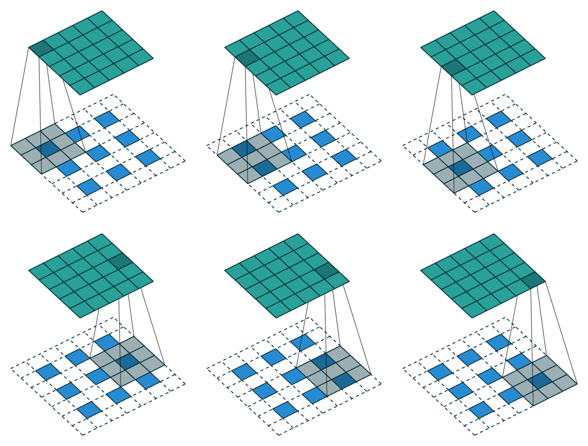
Cover image source: A guide to convolution arithmetic for deep learning - Vincent Dumoulin, Francesco Visin - ArXiv

In ZF Net, the transposed convolution is used to approximate the inverse of convolution, leading to the reconstruction of the activating features from the input image that activates a particular layer. However, strictly speaking, the transposed convolution is not really the inverse of convolution. Then why can it be used to do the reconstruction?

What is transposed convolution

An ordinary convolution can be written in the form of ${Y} = {C} * {X}$. Then the corresponding transposed convolution is defined as:

${X'} = {C}^T * {Y}$

What yields the largest response

The convolution ${Y} = {C} * {X}$ and be transformed to the vectorized form:

$y_i = {c}_i^T {x}$
where ${x}$ is the the flattened input feature map ${X}$, $y_i$ is the $i$-th element of the flattened output feature map ${Y}$, and $c_i$ is the actual weights that are applied to ${x}$ to yield $y_i$.

What will makes $y_i$ generates the largest response? For example, ${x} = (1, 2, -1)$ is a good heuristic when ${c}_i = (1, 2, -1)$, since after the multiplication all negative values in ${c}_i$ becomes positive values. Therefore:

If ${x}$ can not be arbitrarily big, then setting ${x} = {c}_i$ yields the largest value of $y_i$. Or we can say, setting ${x} = {c}_i$ yields the largest response in the $i$-th item of the flattened output feature map ${Y}$.

Back-props the feature map

Now let's return to ZF Net's scenario: we know the response feature map ${Y}$, what kind of input feature map ${X}$ that is most activating to generate ${Y}$?

We have known that ${x} = {c}_i$ yields the largest value of $y_i$. However, the value (aka. activating level) of $y_i$s are different. So a intuitive idea is using $y_i$ as the weight to constitute the desirable ${x}$:

${x'} = \sum_i y_i {c}_i$
${X'} = {C}^T * {Y}$

That's exactly a transposed convolution of ${C}$!

Visualization of transposed convolution

In previous discussions, the transposed convolution is converted to the flatten vectorized form, which may be a little bit confusing. However, the vectorized form can always be stacked back to the matrix form, which leads to the conclusion that a transposed convolution is actually an ordinary convolution but padding the original ${X}$ inside and outside with the stride, as shown below:

Image source: A guide to convolution arithmetic for deep learning - Vincent Dumoulin, Francesco Visin - ArXiv

This makes the implementation of transposed convolution very simple, as in:

ConvTranspose2d — PyTorch 2.2 documentation