





Understanding Deep Learning | Simon J.D. Prince
Free official electronic version: Understanding Deep Learning
P.S. This note won't cover the basics. Instead, I will focus on nuances that basic textbook won't cover. As the book title suggests, this book is for those who want to gain a deeper understanding of why and how deep learning works. To be honest, I have learned through these basic network architectures multiple times, both from textbooks and some of the original papers. But there are still lots of things I found intriguing and sometimes even surprising.
P.S. Parts and chapters are renamed and reshuffled. I will first summarize major network architectures, which are versatile and somehow swappable components. Then I will iterates through major learning paradigms: from basic supervised training, to unsupervised (generative) learning, then to reinforcement learning. This order may be logical for note taking, but not for a learner who's not familiar with these contents.
Part I. Major network architectures
Fully connected layers / multi-layer perceptron (MLP)
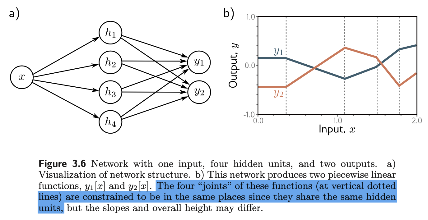
- A single fully connected layer (a.k.a multi-layer perceptron, MLP) is composed of: (i) a linear mapping from input nodes to hidden units, (ii) a second linear mapping from hidden units to output nodes, (iii) activation on each output nodes
The universal approximation theorem proves that for any continuous function, there exists a shallow network that can approximate this function to any specified precision
- For each output node, when there are hidden units and the activation is ReLU, the output is a sum of ReLU functions, each with a different slope and joint, forming a function with at most linear regions
- Since all output nodes share the same hidden units, their linear regions have the same joints but different slopes
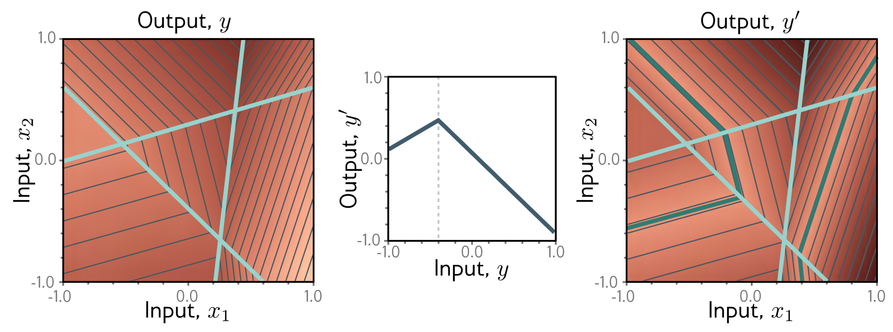
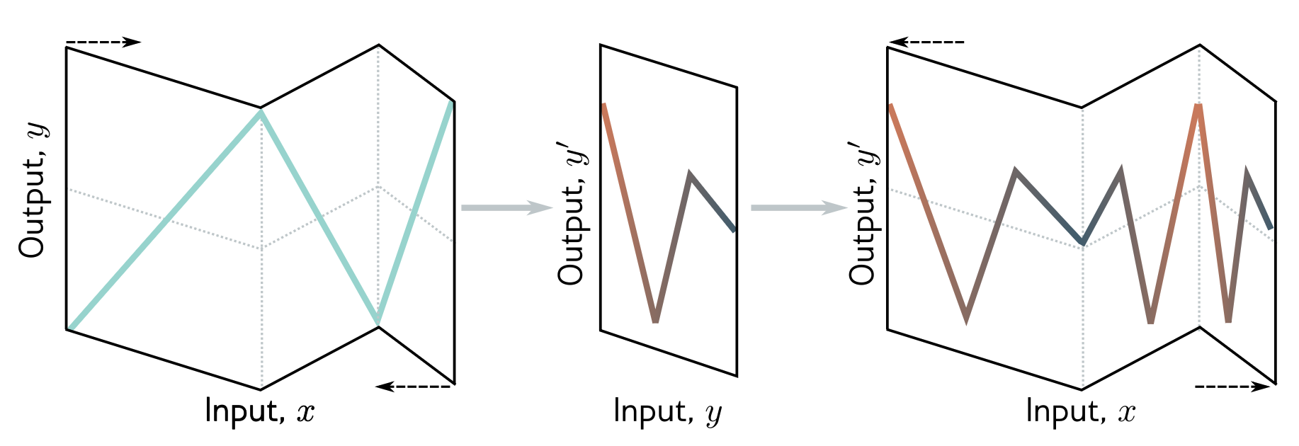
- When multiple layers are stacked, the networks become "deep". We can think of it in two ways: (i) since each layer is a piecewise linear function with multiple linear regions, layering another layer upon it further segments each region into even more linear regions, thus increasing the expressivity of the network; (ii) however, the segmenting of each region is not independent, rather, they share symmetry since each are segmented by the same next layer, which creates a "folding" like pattern
- Deeper networks are usually easier to train (than a wider one with the same number of parameters), possibly due to the fact that over-parameterized deep models have a large family of roughly equivalent solutions that are easy to find
- Deeper networks also seem to generalize better (than a wider one with the same number of parameters), possibly due to the fact that the folding pattern creates a bias towards learning simpler, symmetric functions in each layer
Convolutional neural networks (CNN)
- Underlying idea
However, fully connected networks have no notion of “nearby” and treat the relationship between every input equally... the interpretation of an image is stable under geometric transformations. An image of a tree is still an image of a tree if we shift it leftwards by a few pixels.
- Equivariant
Networks for per-pixel image segmentation should be equivariant to transformations.
- Invariant Likewise, networks for image classification should be invariant to transformations
- Equivariant
- Pipeline
To achieve equivariance, a CNN uses convolution as its main operation, applying the same kernel to all locations of the input. For each input channel, multiple kernels produce multiple (hidden) maps. Note that kernels for different channels don't share weights. The maps from all input channels are then weighted and summed (with bias and activation) to produce multiple output channels—just like the weighted summation (with bias and activation) of hidden units to produce multiple output nodes in an MLP
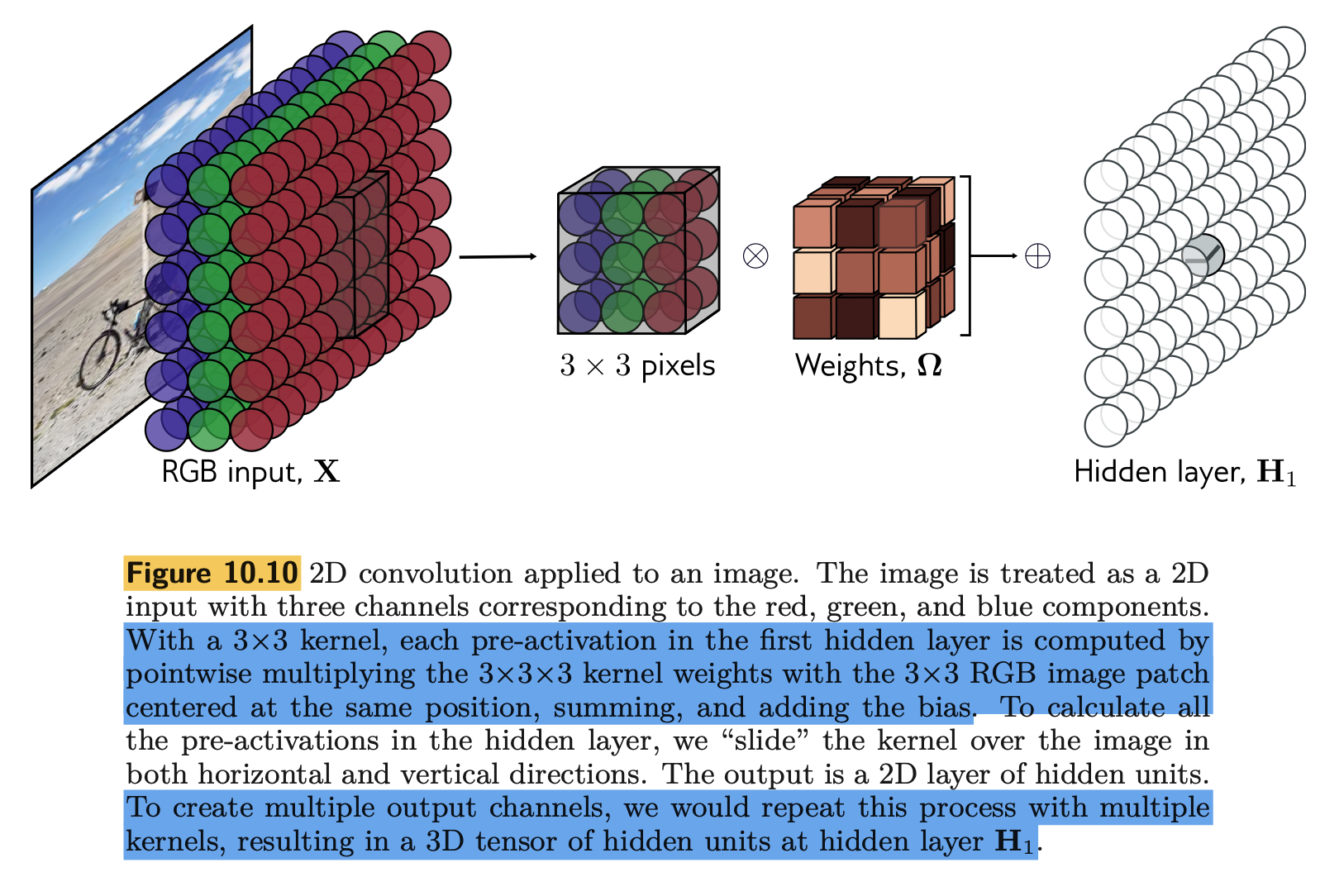
- Parameters of convolution
Padding, stride, kernel size, dilation rate - Downsampling
Stride, max pooling, mean pooling, average pooling, etc. - Upsampling
Direct duplication, max unpooling, bilinear interpolation, transposed convolution, etc. - Change channel number
The kernel size determines the receptive field of the convolution, while the number of weighted sums (with bias and activation) determines the number of output channels. To change the number of channels, we can use a 1x1 convolution, which is equivalent to a fully connected layer applied to each pixel independently
- Parameters of convolution
Residual networks (ResNet)
- Issues with deeper networks
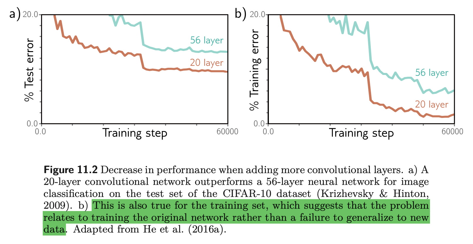
- Shattered gradients
Since tiny changes to early layers could cause big changes to the later layers, the gradients would appear to be "shattered" - Vanishing gradients
If a signal is clipped by an activation layer, the gradients won't pass through this layer when they propagate backward. As the number of layers increases, the probability of vanishing gradients increases, making the network hard to train - Exploding gradients
If the weights are initialized with a large variance, the output of each layer would have a larger variance than the input. As the number of layers increases, the variance of the output would explode, making the network hard to train
- Shattered gradients
- Residual connections
The residual blocks branch from the input and then add back to it, causing the blocks to learn the "residual" rather than full transformations of the input signal

- Benefits
They create multiple (and shorter) paths from the first layer to the final output, making gradients easier to back-propagate through
Also, learning small residuals is easier than learning full transformations, especially when the identity mapping is a good approximation of the desired transformation
- Order of operations in the residual blocks
[!tip]
The common practice in an MLP is to place a linear layer before activation. However, in a residual block, this makes the added residual entirely positive. Therefore, the activation should be placed before the linear layer.
But that introduces another problem: if the input to the first layer is entirely negative, the activation in the first residual block will clip it to zero. Therefore, a linear layer should be placed before all residual blocks
- Benefits
- Exploding variance with residual blocks
If the input signal has variance 1, then after the first residual block, the variance would be 2 since the original signal and the residuals are added. After the next residual block, the variance would be 4, and so on... To address this issue, the common practice is to use batch normalization- BatchNorm
For each input channel, compute the mean and standard deviation across the batch and use them to shift and scale the input. A learned scale and a bias are then applied to preserve a learnable scale and bias while maintaining stability across all layers
P.S. In image processing, the mean and standard deviation are computed for each image channel across the batch.
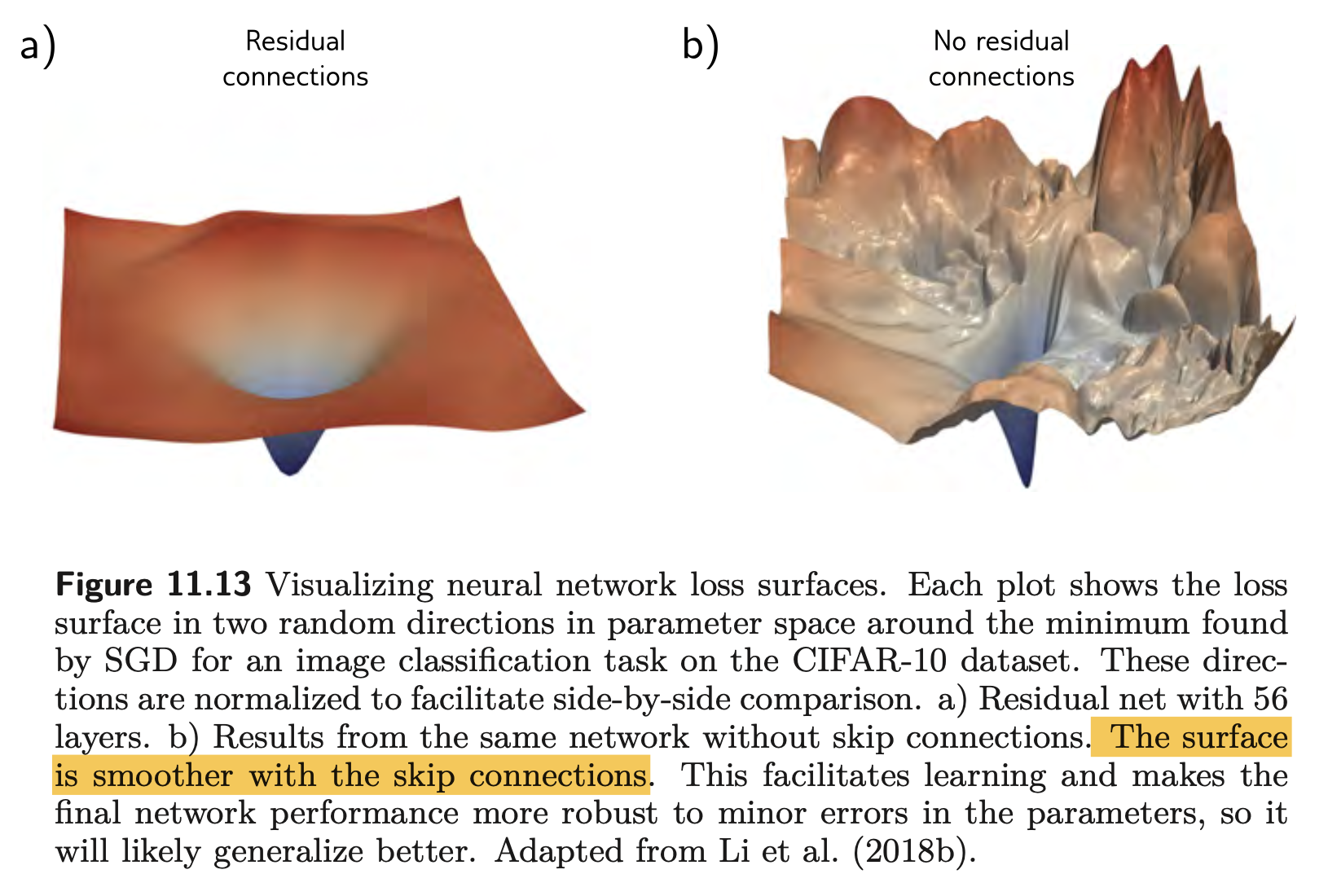
P.S. With residual blocks and BatchNorm, each residual block adds only variance 1 if the learned . This makes the loss surface smoother. The normalization also makes large groups of model weights equivalent, making it easier to reach a good minimum. - Other normalization schemes
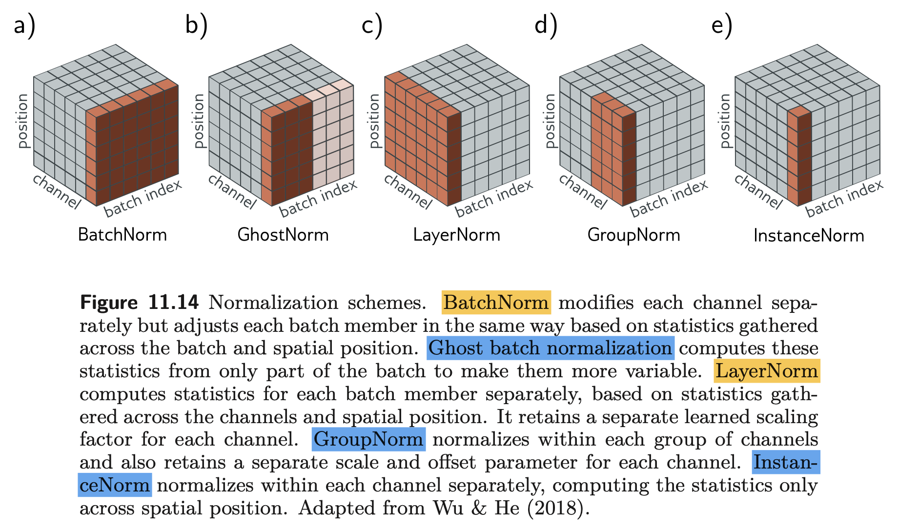
- BatchNorm
Transformers
-
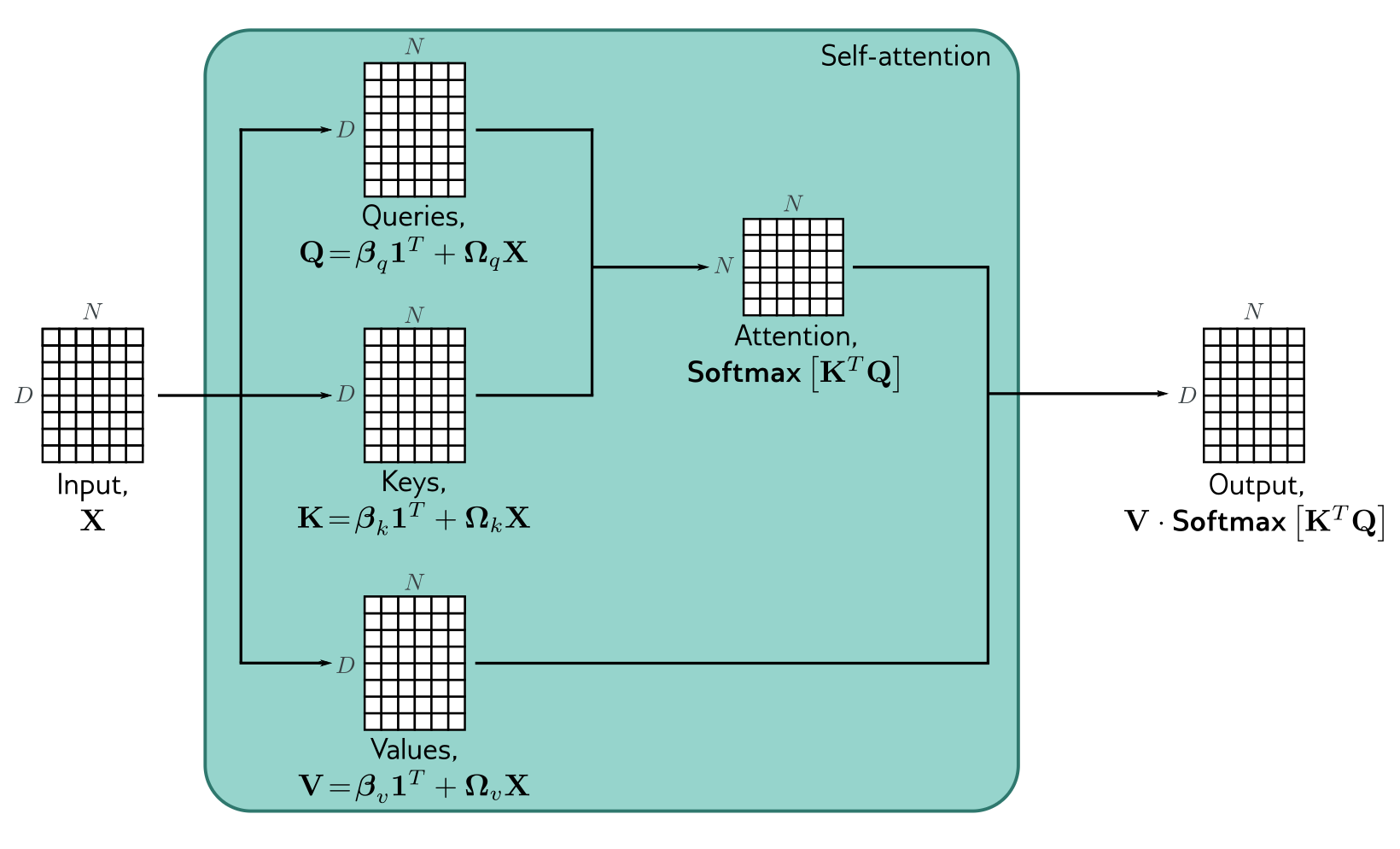
Dot-product self-attention
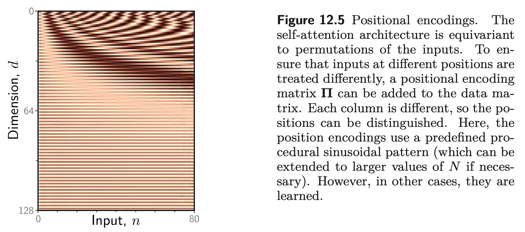
- Positional encoding
- Scaled dot-product self-attention
The dot products in the attention computation can have large magnitudes and move the arguments to the softmax function into a region where the largest value completely dominates. Small changes to the inputs to the softmax function now have little effect on the output (i.e., the gradients are very small), making the model difficult to train. To prevent this, the dot products are scaled by the square root of the dimension of the queries and keys (i.e., the number of rows in and , which must be the same):
- Multi-head attention
The -dimensional input is split into heads, each of which has dimensions. Each head has its own learned , , and . The outputs of all heads are concatenated into a -dimensional representation and then projected with a learned .
- Positional encoding
-
Transformer
- Typical Transformer layers
- Other components
- Tokenization
- Embeddings
- Encoder-decoder: BERT
- Decoder-only: GPT
- Masked self-attention
For language modelling, an attention mask is typically applied to the attention weights to prevent the model from attending to future tokens. This is done by adding a large negative value (e.g., ) to the attention weights corresponding to future tokens before applying the softmax function, effectively setting their attention weights to zero.[!important]
During training, each token only attends to the previous tokens and predicts the next token. Therefore, the model predicts a series of prediction tasks in one go, making the training very efficient.During inference, since future tokens won't affect current tokens' keys and values, they can be cached and reused for the next token's attention computation, which makes the inference more efficient.
- Masked self-attention
- Transformers for images
Vision Transformer (ViT) 👉 Swin Transformer 👉 etc.
- Typical Transformer layers
Graph neural network (GNN)
- Graph representation
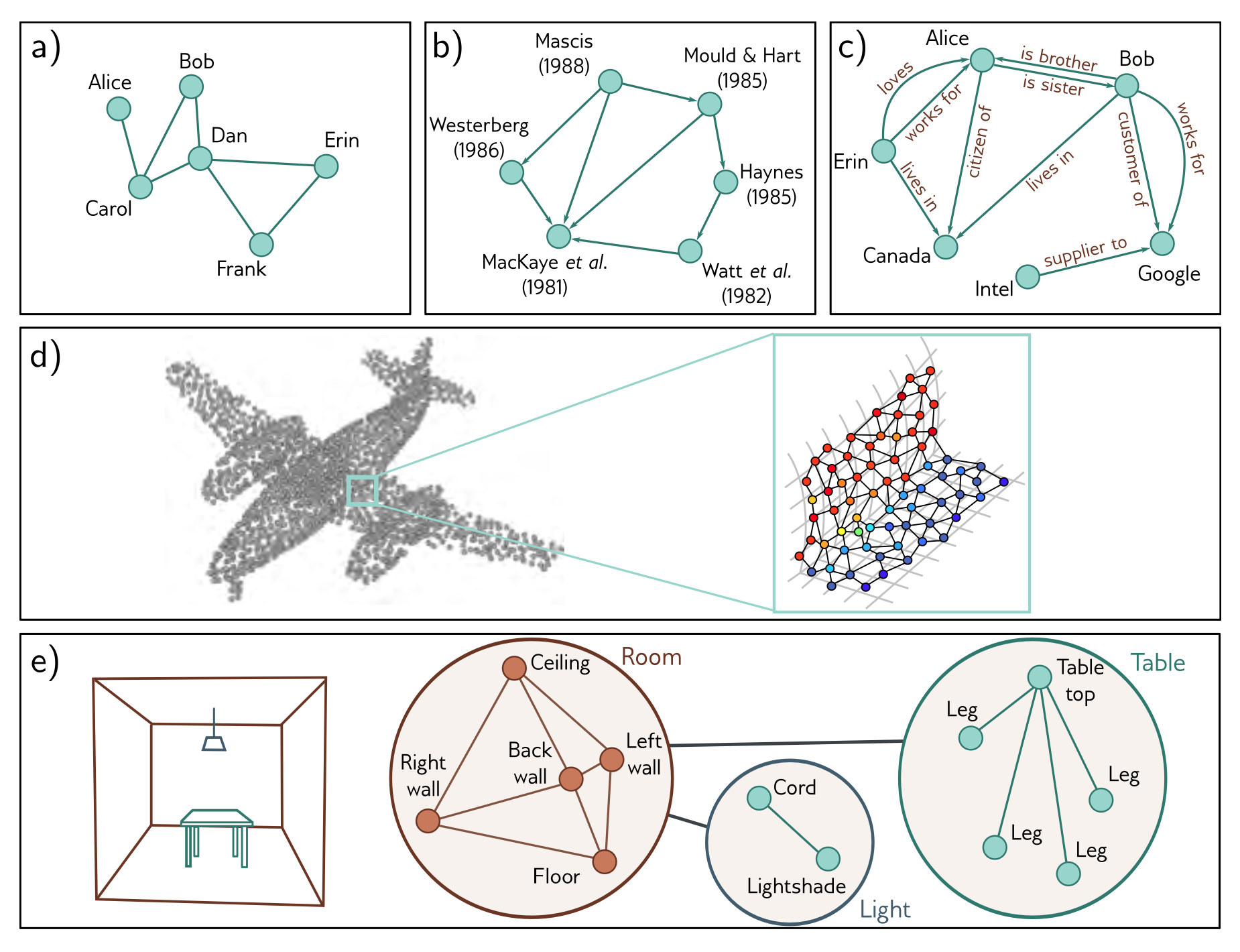
- Node embedding
- Edge embedding
- Adjacency matrix
Position of the adjacency matrix contains the number of walks of length one from node to node . The entry at position of contains the number of unique walks of length from node to node .
P.S. This is not the same as the number of unique paths since the walks include routes that visit the same node more than once. Nonetheless, a non-zero entry at position indicates that the distance from to must be less than or equal to .
- Graph neural networks (GNNs)
A graph neural network is a model that takes the node embeddings and the adjacency matrix as inputs and passes them through a series of layers. The node embeddings are updated at each layer to create intermediate “hidden” representations before finally computing output embeddings .
- Tasks
- Graph-level
For graph-level tasks, the output node embeddings are combined (e.g., by averaging), and the resulting vector is mapped via a linear transformation or neural network to a fixed-size vector.
- Node-level
The final node embeddings can be used for node-level prediction. - Edge-level
A graph can be converted to its edge graph, where nodes become edges and edges become nodes, thus converting edge-level tasks into node-level tasks.
- Graph convolutional networks (GCNs)
These models are convolutional in that they update each node by aggregating information from nearby nodes. As such, they induce a relational inductive bias (i.e., a bias toward prioritizing information from neighbors). They are spatial-based because they use the original graph structure. This contrasts with spectral-based methods, which apply convolutions in the Fourier domain.
- Mean/max pooling aggregation
- Attention-based aggregation
The attentions are masked so that each node only attends to itself and its neighbors
- Kipf normalization
In Kipf normalization, the sum of the node representations is normalized as:
with the logic that information coming from nodes with a very large number of neighbors should be down-weighted since there are many connections and they provide less unique information. This can also be expressed in matrix form using the degree matrix:
- Residual connections
With residual connections, the aggregated representation from the neighbors is transformed and passed through the activation function before summation or concatenation with the current node.
- Batch sampling
- Neighborhood sampling
Start with the batch nodes and randomly sample a fixed number of their neighbors in the previous layer. Then, we randomly sample a fixed number of their neighbors in the layer before, and so on.
- Graph partitioning
Cluster the original graph into disjoint subsets of nodes and sample from these clusters to maximize the number of internal links.
- Neighborhood sampling
- Tasks
Part II. Supervised learning
Loss functions
To derive the loss function from the maximum likelihood perspective:
[!important]
- Choose a suitable probability distribution defined over the domain of the predictions with distribution parameters .
- Set the machine learning model to predict one or more of these parameters, so and .
P.S. Usually the predicted parameter is the mean of the Gaussian distribution.- To train the model, find the network parameters that minimize the negative log-likelihood loss function over the training dataset pairs :
P.S. The underlying assumption is that the training data samples are independent and identically distributed (i.i.d.), so that . Therefore, taking the negative log likelihood yields (5.6).
4. To perform inference for a new test example , return either the full distribution or the value where this distribution is maximized.
P.S. When the predicted parameter is the mean of the Gaussian distribution, the mean would be the value where the distribution is maximized; thus it's equivalent to taking the network output as the value directly.
P.S. Here we derive the loss function from the perspective of maximizing likelihood or minimizing negative log likelihood. Another approach, called cross-entropy loss, is minimizing the Kullback-Leibler (KL) divergence between the empirical data distribution and the model distribution. They are mathematically equivalent.
- Regression 👉 Least squares loss
[!note]
We use a normal distribution as the probability model and let the neural network predict the mean:Then we derive the least squares loss function:
- Classification 👉 Cross-entropy loss
- Binary classification 👉 Binary cross-entropy loss
[!note]
We use a Bernoulli distribution as the probability model and let the neural network predict the probability of the positive class :where . Then we derive the binary cross-entropy function:
- Multi-class classification 👉 Multi-class cross-entropy loss
[!note]
We use a categorical distribution as the probability model and let the neural network predict the probability of each class :where . Then we derive the multi-class cross-entropy function:
- Binary classification 👉 Binary cross-entropy loss
Fitting models
- Gradient descent
Step 1. Compute the derivatives of the loss with respect to the parameters:
Step 2. Update the parameters according to the rule:
where the positive scalar determines the magnitude of the change. The first step computes the gradient of the loss function at the current position. This determines the uphill direction of the loss function. The second step moves a small distance downhill (hence the negative sign).
- Local minima
Zero gradient (update stops), loss increases in all directions, but not necessarily the lowest loss - Saddle points
Zero gradient (update stops), loss increases in some directions and decreases in others
- Local minima
- Stochastic gradient descent (SGD)
To escape local minima, we can introduce randomness into the optimization process by selecting a subset of data samples at each iteration:The mechanism for introducing randomness is simple. At each iteration, the algorithm chooses a random subset of the training data and computes the gradient from these examples alone. This subset is known as a minibatch or batch for short. The update rule for the model parameters at iteration is hence:
where is a set containing the indices of the input/output pairs in the current batch and, as before, is the loss due to the pair. The term is the learning rate... A single pass through the entire training dataset is referred to as an epoch.
- Momentum term
A common modification to stochastic gradient descent is to add a momentum term. We update the parameters with a weighted combination of the gradient computed from the current batch and the direction moved in the previous step:
where is the momentum (which drives the update at iteration ), controls the degree to which the gradient is smoothed over time, and is the learning rate.
- The gradient step is an infinite weighted sum of all the previous gradients
- The effective learning rate increases if all these gradients are aligned over multiple iterations
- The effective learning rate decreases if the gradient direction repeatedly changes as the terms in the sum cancel out
- The overall effect is a smoother trajectory and reduced oscillatory behavior in valleys
- Momentum term
- Adaptive gradient momentum (Adam)
-
Motivation
Adam addresses one core issue of SGD:[!warning]
When the gradient of the loss surface is much steeper in one direction than another, it is difficult to choose a learning rate that (i) makes good progress in both directions and (ii) is stable. -
How it works
The core idea is to divide the gradient by its square root, so that the step lengths are normalized. To make it adaptive, both the gradient and the squared gradient are estimated using momentum:where and are the momentum coefficients for the two statistics.
Using momentum is equivalent to taking a weighted average over the history of each of these statistics. At the start of the procedure, all the previous measurements are effectively zero, resulting in unrealistically small estimates. Consequently, we modify these statistics using the rule:
Since and are in the range , the terms with exponents become smaller with each time step, the denominators become closer to one, and this modification has a diminishing effect.
Finally, we update the parameters as before, but with the modified terms:
The result is an algorithm that can converge to the overall minimum and makes good progress in every direction in the parameter space.
-
Visualization
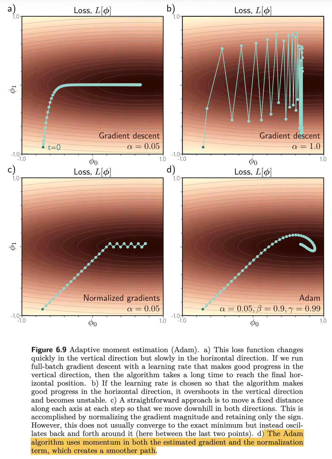
-
Backward propagation
The aforementioned optimization algorithms rely on the computation of , which can be efficiently computed using the backward propagation algorithm. The key idea is to apply the chain rule of calculus to compute the gradient of the loss function with respect to each parameter in the network, starting from the output layer and moving backward through the network:
where and are arbitrary intermediate layer outputs that depend on . By recursively applying this process, we can compute the gradients for all parameters in the network.
He initialization
Assuming that the distribution of pre-activations at the previous layer is symmetric about zero, half of these pre-activations will be clipped by the ReLU function, and the second moment will be half the variance of (see problem 7.14):
This, in turn, implies that if we want the variance of the subsequent pre-activations to be the same as the variance of the original pre-activations during the forward pass, we should set:
where is the dimension of the original layer to which the weights were applied. This is known as He initialization.
Regularization
-
Explicit regularization
The regularization term can be considered as a prior that represents knowledge about the parameters before we observe the data and we now have the maximum a posteriori or MAP criterion:
moving back to the negative log-likelihood loss function by taking the log and multiplying by minus one, we see that .
-
L2 regularization (weight decay)
The most commonly used regularization term is the norm, which penalizes the sum of the squares of the parameter values:
... Here, the regularization term will favor functions that smoothly interpolate between the nearby points. This is reasonable behavior in the absence of knowledge about the true function.
[!important]
L2 regularization is usually only applied to the weights of the network, not the biases. Smaller weights contribute to smallness, whereas preferring smaller biases could risk underfitting the data. Therefore, L2 regularization is also called weight decay. -
L0 regularization
The L0 regularization term applies a fixed penalty for every non-zero weight. The effect is to “prune” the network. L0 regularization can also be used to encourage group sparsity... L0 regularization is challenging to implement since the derivative of the regularization term is not smooth, and more sophisticated fitting methods are required.
-
L1 regularization
Somewhere between L2 and L0 regularization is L1 regularization or LASSO (least absolute shrinkage and selection operator), which imposes a penalty on the absolute values of the weights.
-
-
Implicit regularization
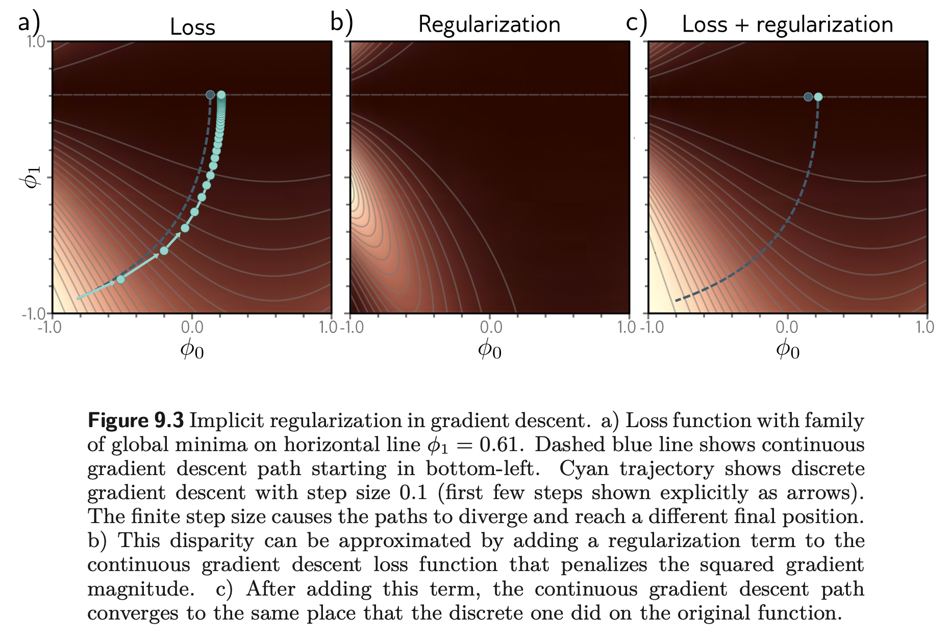
- Gradient Descent (GD)
The trajectory of gradient descent will be affected by the step size. The trajectory of a continuous version of GD with an infinitesimally small step size can be described by , while the discrete version of GD can be described by . If we "simulate" the discrete version of GD with the continuous one by modifying the loss function, the modified loss is: Therefore, discrete GD repels the trajectory toward a path with smaller gradient norm, which is a form of implicit regularization. - Stochastic Gradient Descent (SGD) where is the loss for the -th of the batches in an epoch. Compared with GD, it further repels the trajectory toward a path with smaller gradient variance among batches, which is another form of implicit regularization and might explain why SGD generalizes better than GD, especially with smaller batch sizes.
- Gradient Descent (GD)
Heuristics-driven tricks
Beyond explicit and implicit regularization, there are many heuristics-driven tricks that can influence the learning trajectory or modify the eventual models and thus improve the generalization performance of deep learning models. These include:
- Influencing the learning trajectory
- Dropout
Dropping a random subset of units in the network during training, which forces the network to learn redundant representations (i.e. avoid relying on a few neurons for prediction) and prevents overfitting. During inference, all units are used, but their outputs are scaled by 1 - dropout rate to account for the missing units during training. - Early stopping
Using a validation set to monitor the model's performance during training and stopping the training process when the performance on the validation set starts to degrade, which prevents overfitting to the training data -- as training progresses, the model may start to try to fit the noise in the training data, which makes the function less smooth and can hurt its performance on unseen data. - Transfer learning
Use a model trained on a large dataset for a related task as a starting point for training on a smaller dataset for the target task. This allows the model to leverage the knowledge learned from the large dataset and can improve generalization on the target task, compared with learning from scratch on a small dataset - Multi-task learning
Train a network to perform multiple related tasks simultaneously, which can help the model learn more generalizable features and improve performance on each individual task
- Dropout
- Modifying the dataset
- Applying noise
Adding noise to the input data can help the model learn to be more robust to variations in the input and prevent overfitting. This can be done by adding Gaussian noise, randomly flipping or rotating images, or randomly masking parts of the input. - Label smoothing
A technique where the label distribution (e.g. class label, language token, etc.) is smoothed by assigning a small probability to all classes, rather than assigning a probability of 1 to the correct class and 0 to all others. This prevents the model from becoming overconfident in its predictions and can improve generalization - Data augmentation
Manipulating the data to generate new training examples, which can help the model learn to be more robust to variations in the input and prevent overfitting. This can be done by applying transformations such as rotation, scaling, flipping, or cropping to images, or by adding noise or perturbations to text or audio data
- Applying noise
- Ensembling
Combining the predictions of multiple models to improve overall performance and reduce overfitting. This can be done by averaging the predictions of multiple models, or by using a more sophisticated method such as stacking or boosting
Evaluation
To fairly evaluate the performance of a model, we need to split the dataset into three disjoint sets: training set, validation set, and test set. The training set is used to train the model, the validation set is used for hyperparameter tuning or early stopping, and the test set is used to evaluate the final performance of the model. It's important that the test set is not used during training or hyperparameter tuning to ensure an unbiased estimate of the model's generalization performance.
The following is some mathematical and empirical analysis of the test-set performance.
-
Noise, bias, and variance
We assume the training dataset is sampled stochastically: for an input , the output has the expectation and variance . The expected model that can be learned given all possible training datasets is . Then the expected test-set error over all possible training datasets is:- The variance is uncertainty in the fitted model due to the particular training dataset sampled
The difference between the fitted model under the current training set and the expected learned model given all possible training setsIt follows we can reduce the variance by increasing the quantity of training data. This averages out the inherent noise and ensures that the input space is well sampled.
- The bias is the systematic deviation of the model from the mean of the function we are modeling
The difference between the outputs of the expected learned model given all possible training sets and the actual expected outputThis suggests that we can reduce this error by making the model more flexible. This is usually done by increasing the model capacity.
- The noise is the inherent uncertainty in the true mapping from input to output
The variance in the output during data sampling
- The variance is uncertainty in the fitted model due to the particular training dataset sampled
-
Bias-variance trade-off
For a fixed-size training dataset, the variance term typically increases as the model capacity increases. Consequently, increasing the model capacity does not necessarily reduce the test error. This is known as the bias-variance trade-off.
-
Double descent
However, empirical evidence shows that the test error can decrease again as the model capacity increases beyond a certain point, leading to a double descent curve. This phenomenon is not yet fully understood, but it suggests that over-parameterized models can generalize well despite having low bias and high variance.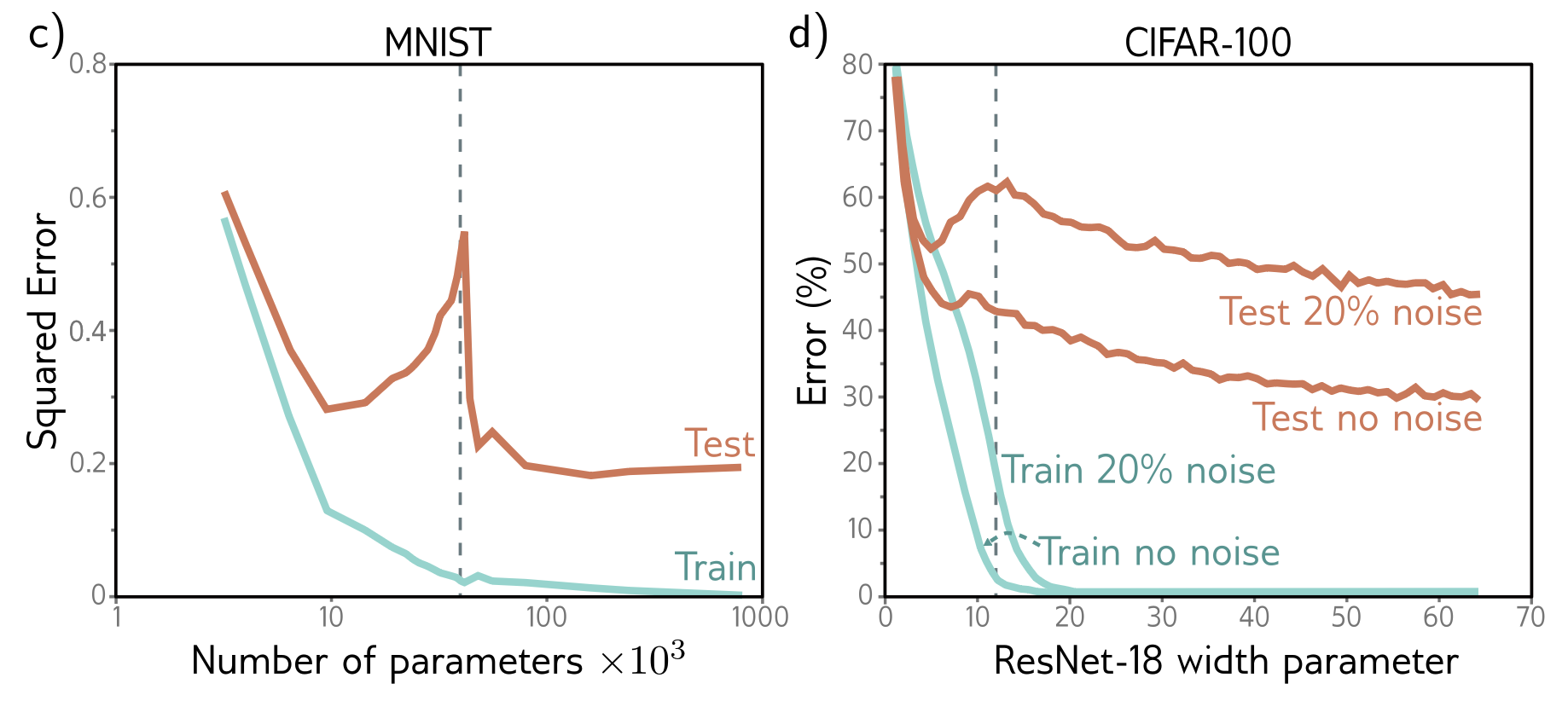
As shown in the figure, as the model capacity increases, the test error first decreases (due to reduced bias), then increases (due to increased variance), and finally decreases again, possibly due to the model's ability to interpolate the training data more smoothly and find a simpler solution that generalizes well.
-
Part III. Unsupervised (generative) learning
[!tip]
Unsupervised learning
├── Clustering / density estimation / dimensionality reduction
├── Generative modeling: VAEs, GANs, diffusion models
└── Self-supervised representation learning: contrastive learning, masked prediction, next-token prediction
Self-supervised learning is a subset of unsupervised learning. Both learn from unlabelled data, by manipulating the original data in some way and constructing an objective (loss) to train the models. The subtle difference is that self-supervised learning focuses on learning useful & transferable representations from such a constructed task, while the focus of unsupervised learning is broader: e.g., extracting the structure in the dataset, learning a data distribution for generating new samples, etc.
- Latent variable
A latent variable can be considered a compressed version of a data example x that captures its essential qualities
- Self-supervised learning
- Contrastive
In contrastive self-supervised learning, the model is trained to distinguish between similar and dissimilar pairs of data points. This encourages the model to learn representations that capture the underlying structure of the data and can improve generalization on downstream tasks. - Generative
In generative self-supervised learning, the model is trained to generate or reconstruct the input data from a corrupted version of it. This forces the model to learn useful representations of the data that can be used for downstream tasks.- Probabilistic generative models
\tag{14.1}In addition to generating new examples, they assign a probability to each data point . This will depend on the model parameters , and in training, we maximize the probability of the observed data , so the loss is the sum of the negative log-likelihoods (figure 14.2b):
- Desired properties
Sampling: efficient, high-quality, high-coverage
Latent space: well-behaved, disentangled
Efficient likelihood computation - Metrics
-
Test likelihood
Measure the likelihood assigned to a test dataset. This is not practical for models that cannot compute likelihoods efficiently, such as GANs and diffusion models. -
Inception score (IS)
Use a pre-trained classifier to measure the quality and diversity of generated samples. However, it is only sensible for generative models of the ImageNet database and is sensitive to the particular classification model. Also, it does not reward diversity. -
Fréchet inception distance
Compute a symmetric distance between the distributions of generated samples and real examples. The two distributions are approximated by multivariate Gaussians, and the distance is estimated using the Fréchet distance.it does not model the distance with respect to the original data but rather the activations in the deepest layer of the inception classification network. These hidden units are the ones most associated with object classes, so the comparison occurs at a semantic level, ignoring the more fine-grained details of the images. This metric does take account of diversity within classes but relies heavily on the information retained by the features in the inception network; any information discarded by the network does not contribute to the result.
-
Manifold precision/recall
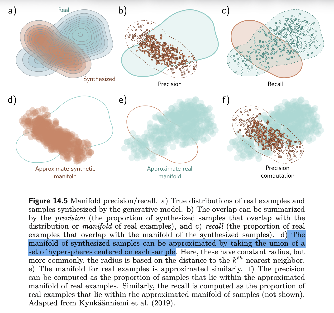
We consider the overlap between the data manifold (i.e., the subset of the data space where the real examples lie) and the model manifold (i.e., where the generated samples lie).
- The precision is the fraction of model samples that fall into the data manifold. This measures the proportion of generated samples that are realistic.
- The recall is the fraction of data examples that fall within the model manifold. This measures the proportion of the real data the model can generate.
-
- Probabilistic generative models
- Contrastive
Next we move on to unsupervised generative learning.
Generative adversarial networks (GAN)
- GAN loss
- : the -th random latent/noise sample, typically drawn from a simple distribution such as
- : the generator with parameters , which maps latent sample to a synthetic data sample
- : the discriminator with parameters , which produces a logit indicating whether is real or generated. Thus can be interpreted as the predicted probability that is real
- The expression inside the brackets is the binary cross-entropy loss for distinguishing real samples from generated samples
- GAN training
The GAN loss can be decomposed into two separate loss functions for the generator and discriminator:- A min-max adversarial game
- The discriminator minimizes with respect to , trying to assign for real data and for generated data.
- The generator maximizes the discriminator's minimum achievable loss with respect to , trying to generate samples that make real and fake data difficult to distinguish.
- At equilibrium, an ideal generator reproduces the real data distribution, so the discriminator can do no better than random guessing:
- Difficulties in GAN training
- Quality v.s. coverage
When the discriminator is optimal, is equivalent to , measuring the alignment between the generated distribution and the real data distribution in terms of both quality and coverage. However, the coverage term doesn't depend on the generator parameters , so the generator only optimizes for quality. This can lead to mode collapse, where the generator produces a limited variety of samples that are of high quality but fail to cover the diversity of the real data distribution. - Vanishing gradients
When the discriminator is too strong, the generator receives very small gradients and struggles to improve. This can lead to slow convergence or failure to learn; on the other hand, if the discriminator is too weak, it cannot provide useful feedback to the generator. A fine balance is needed to ensure that both networks learn effectively.
- Quality v.s. coverage
- Common tricks
- Wasserstein GAN loss
The Wasserstein GAN (WGAN) loss is an alternative formulation of the GAN loss that addresses the vanishing gradient problem by using the Wasserstein distance (also known as Earth Mover's distance) instead of the Jensen-Shannon divergence. - Progressive growing
The generator is initially trained to produce low-resolution images, and the resolution of the generated images is then gradually increased as training progresses. This allows the generator to learn coarse features first and then refine them, leading to more stable training and higher-quality images. - Minibatch discrimination
Make the discriminator aware of the diversity of the minibatch rather than evaluating its samples independently. This encourages the generator to produce a wider variety of samples and helps prevent mode collapse, i.e., exploiting the reward by generating only a few high-quality samples. - Truncation
Sample only latent variables with high probability (i.e., close to the mean).
- Wasserstein GAN loss
- A min-max adversarial game
- Conditional generation
- Conditional GAN
Condition the generation on an attribute vector .
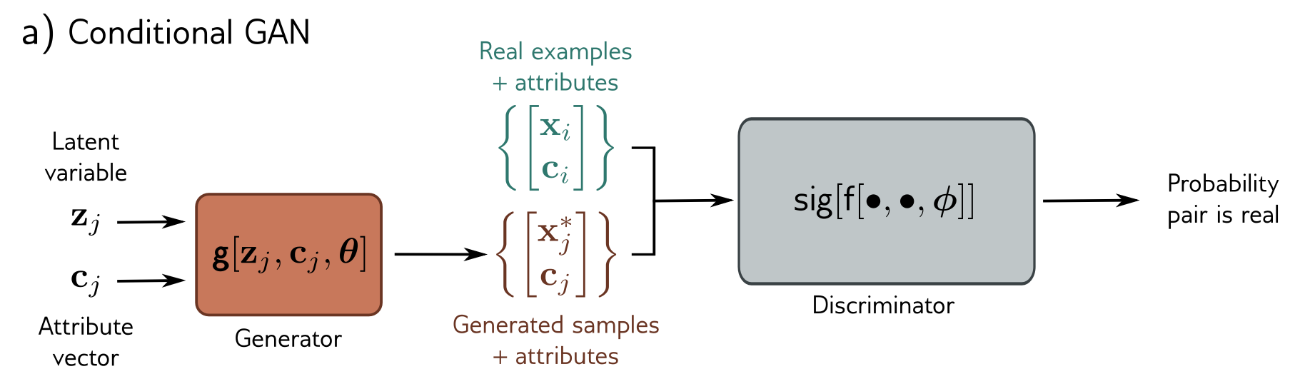
- Auxiliary classifier GAN (ACGAN)
Condition the generation on class and use an auxiliary classifier in the discriminator to predict the class of the generated sample.
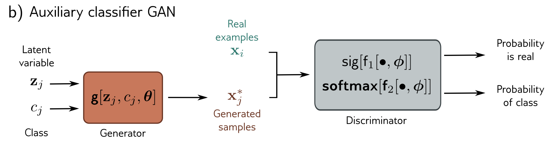
- InfoGAN
Condition the generation on an attribute vector and let the discriminator predict the attribute vector of the generated sample, which encourages the generator to learn disentangled representations of the attributes.
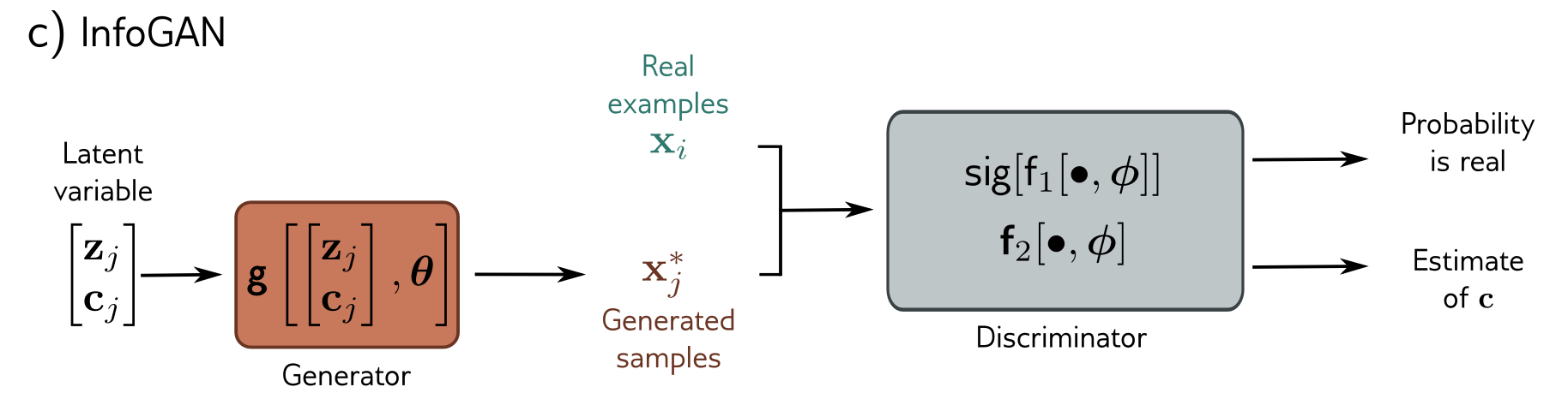
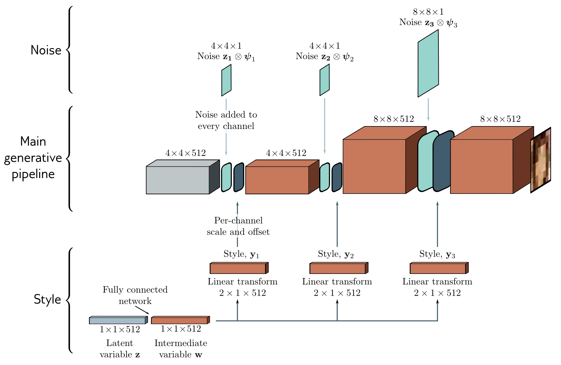
- StyleGAN: separate style from noise
It introduces a set of style and noise latent codes into each layer of the generator, allowing for more control over the generated images and enabling the generation of high-quality images with fine-grained details.
- Conditional GAN
- Image translation
- Pix2Pix
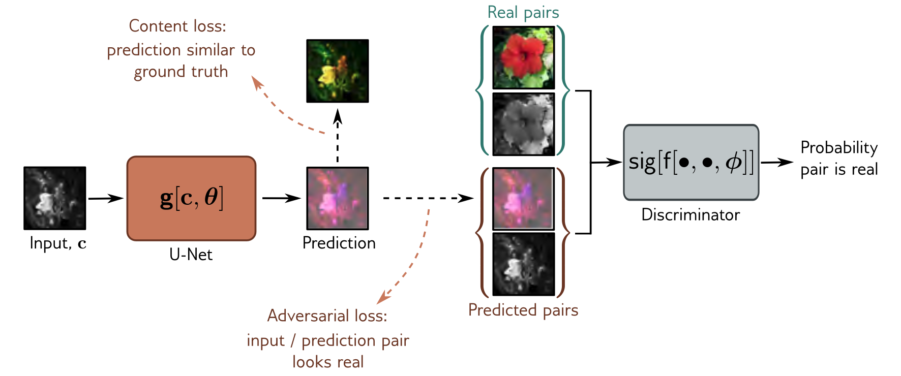
- CycleGAN
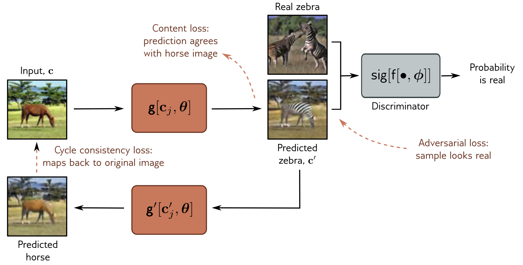
- Pix2Pix
Normalizing flows
Of the four generative models discussed in this book, normalizing flows is the only model
that can compute the exact log-likelihood of a new sample... Normalizing flows can also learn to generate samples that approximate an existing density which is easy to evaluate but difficult to sample from.
-
Mapping from normal distribution to data distribution
The key idea of normalizing flows is to learn a bijective mapping from a simple base distribution (e.g., standard normal) to the complex data distribution. This allows us to compute the exact log-likelihood of a new sample by applying the change of variables formula:where is the latent variable corresponding to the data point , and the determinant term accounts for the volume change under the transformation.
More precisely, the probability of data under the transformed distribution is:
P.S. The density of a distribution is stretched by with high-slope and vice verse.
...
To learn the distribution, we find parameters that maximize the likelihood of the training data or equivalently minimize the negative log-likelihood:where we have assumed that the data are independent and identically distributed in the first line and used the likelihood definition from equation 16.1 in the third line.
-
Invertible network layers
- Linear flows
This is the simplest invertible layer, but it has limited expressiveness: - Elementwise flows
Applies element-wise invertible transformations to achieve non-linearity. However, the elements can't interact with each other. - Coupling flows
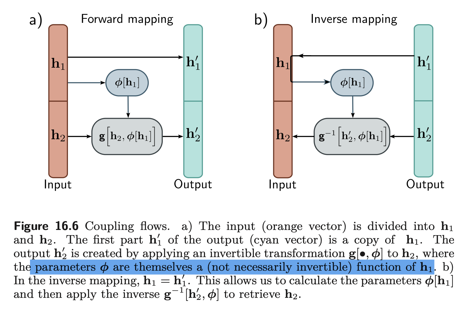
- Autoregressive flows
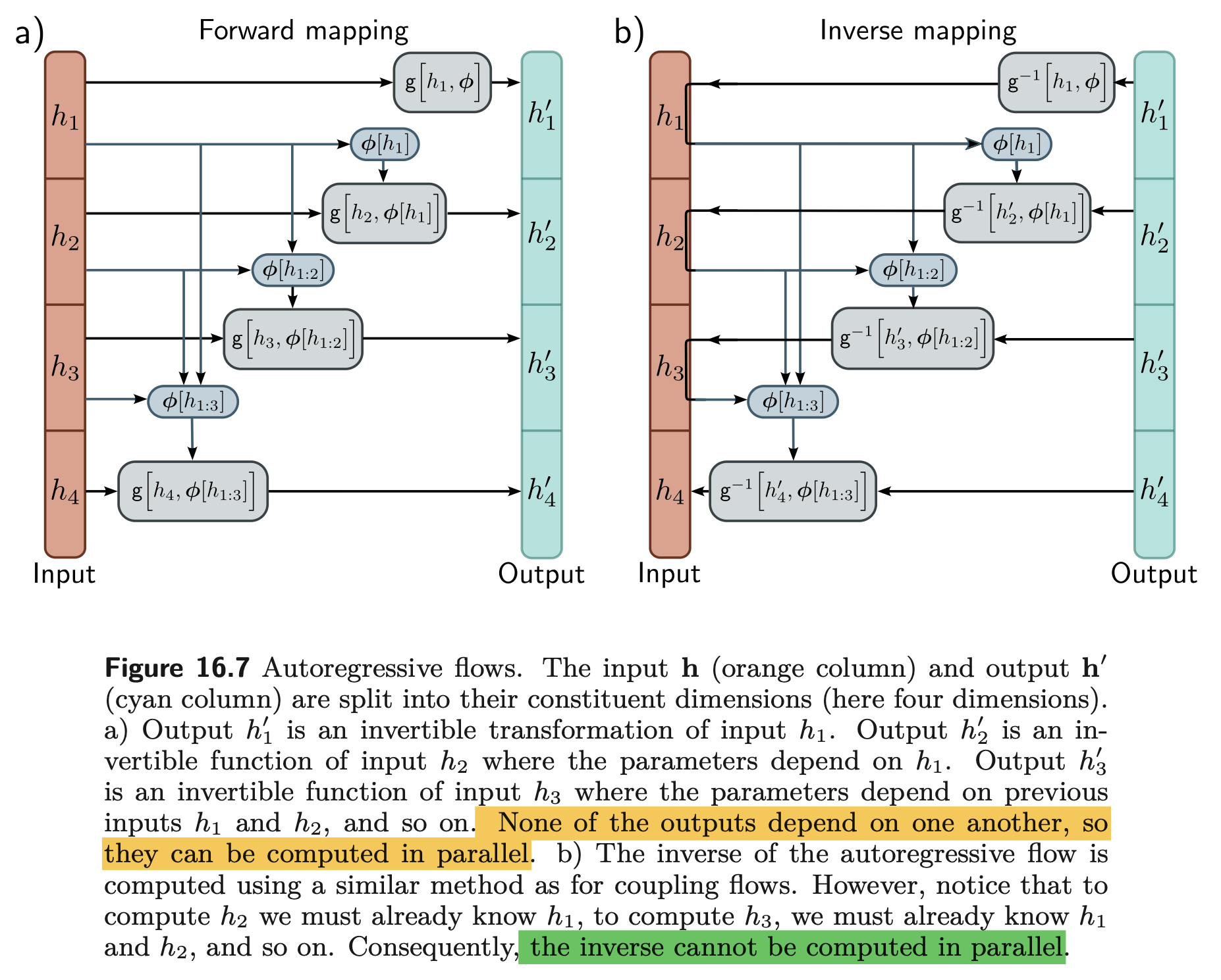
- Residual flows
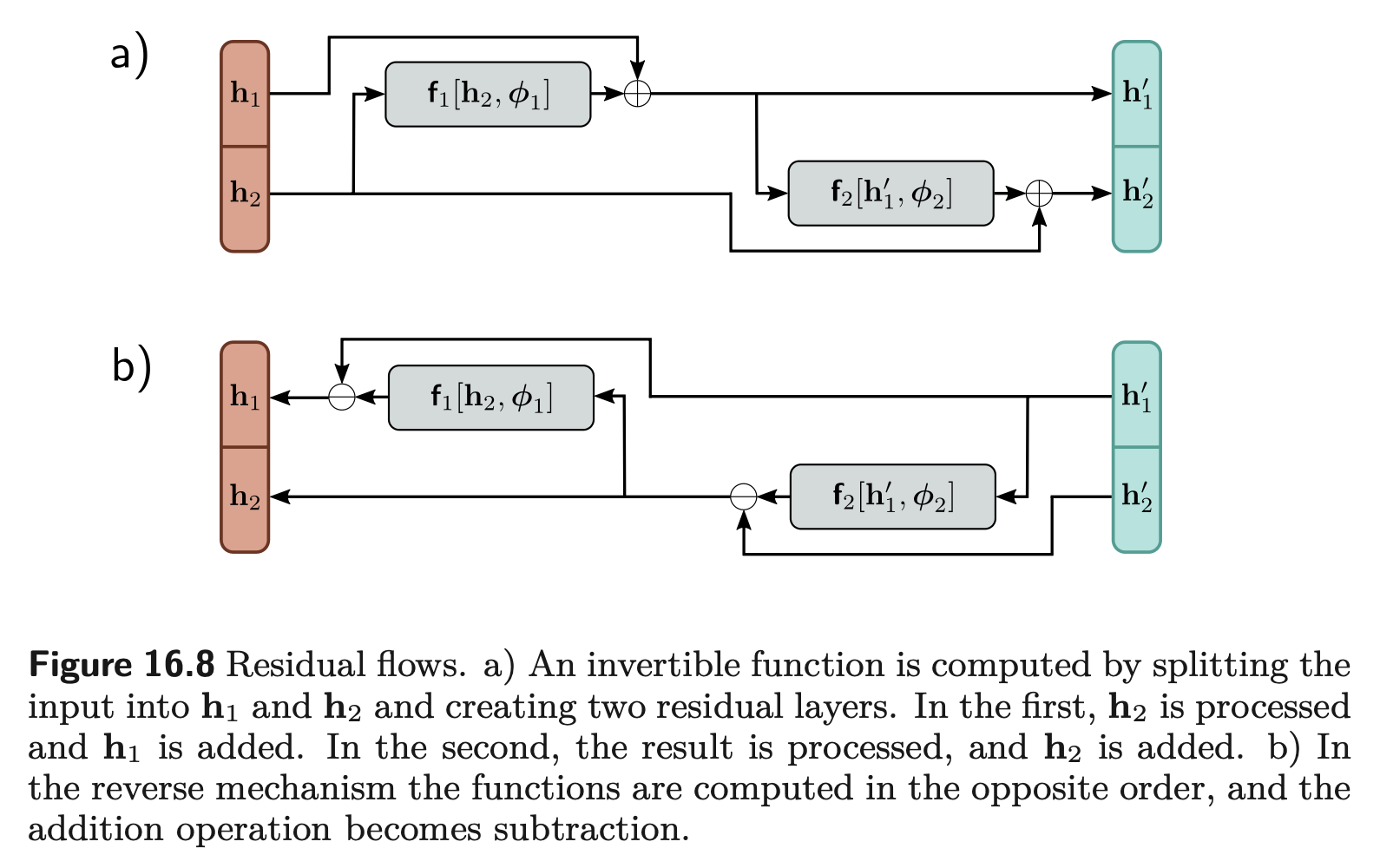
- Multi-scale flows
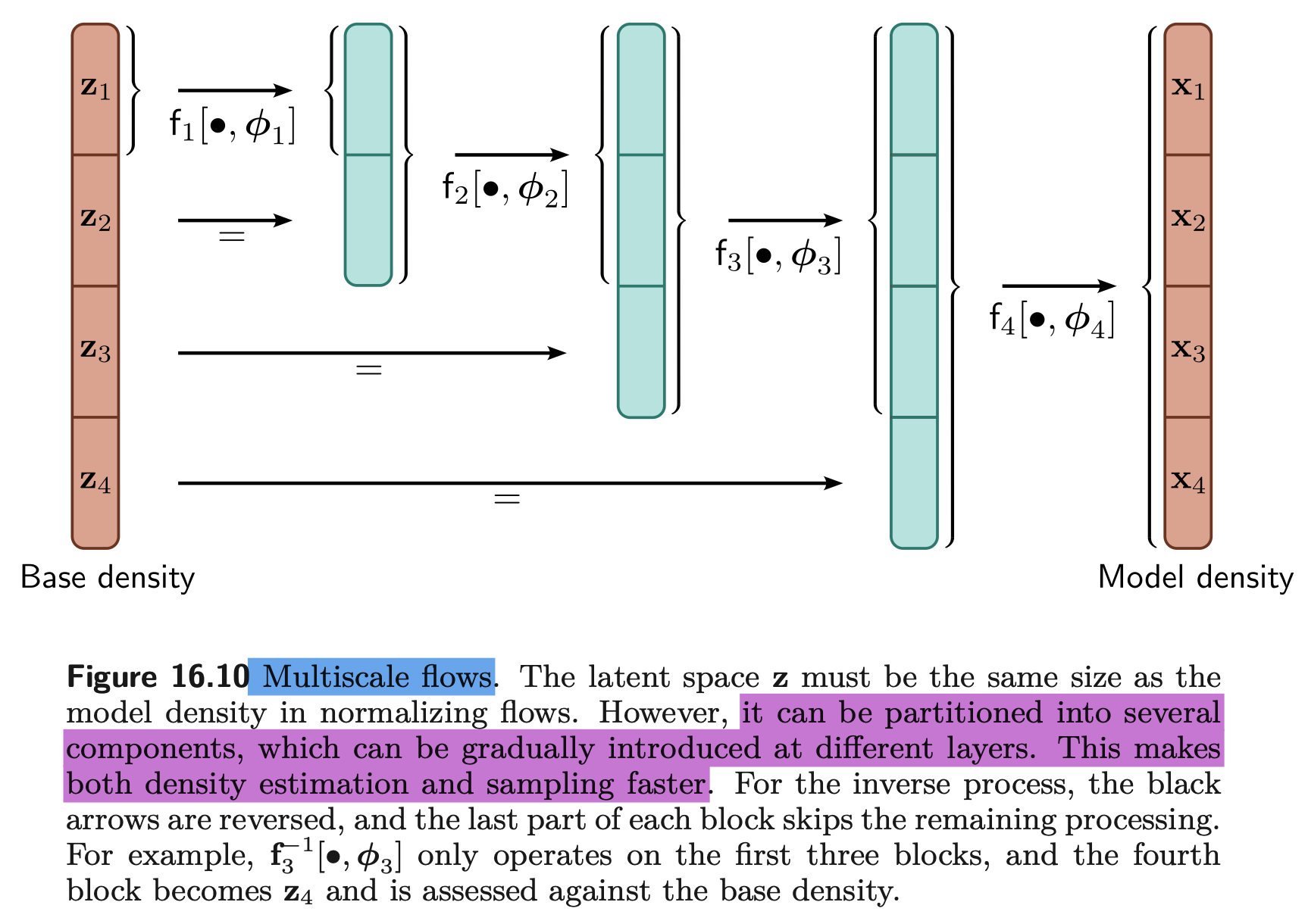
- Linear flows
Variational autoencoders (VAE)
-
Latent variable models
To describe the distribution :is the latent variable, which is usually a standard multivariate normal distribution. is the likelihood of the data given the latent variable, which is usually modeled by a neural network, which predicts the mean of a Gaussian:
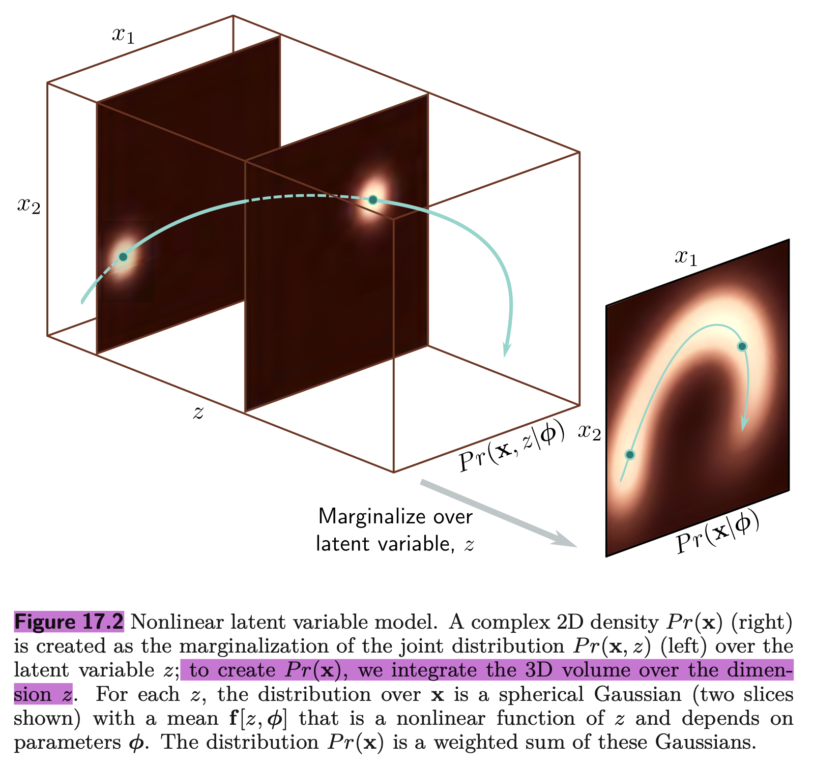
- Ancestral sampling
For generation, we first sample from the prior , and then sample from the likelihood- Evidence lower bound (ELBO)
We start by multiplying and dividing the log-likelihood by an arbitrary probability distribution over the latent variables:
We then use Jensen's inequality for the logarithm (equation 17.12) to find a lower bound:
where the right-hand side is termed the evidence lower bound or ELBO. It gets this name because is called the evidence in the context of Bayes' rule (equation 17.19). In practice, the distribution has parameters , so the ELBO can be written as:
-
Tightness interpretation
The bound will be tight when .
-
Reconstruction interpretation
The first term measures the average agreement between the latent variable and the data, i.e., the reconstruction accuracy; the second term measures the degree to which the auxiliary distribution matches the prior.
-
- Evidence lower bound (ELBO)
- Ancestral sampling
-
Variational autoencoder (VAE)
(17.18) was used to construct the VAE loss:For a very approximate estimate, we can just use a single sample from :
The second term is the KL divergence between the variational distribution
and the prior
The KL divergence between two normal distributions can be calculated in closed form.
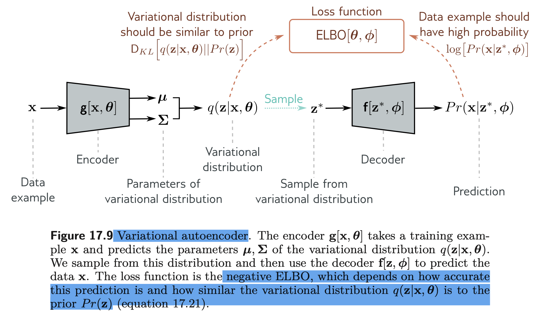
- Encoder
Here, was adapted as since the ELBO will be tight when , which requires the auxiliary distribution to take as input. It is effectively an encoder that maps the data to a latent variable .- Reparameterization
It is difficult to differentiate through this stochastic component... Fortunately, there is a simple solution; we can move the stochastic part into a branch of the network that draws a sample from and then use the relation:
to draw from the intended Gaussian. Now we can compute the derivatives as usual.
- Decoder
The decoder is the likelihood , which maps the latent variable back to the data space and calculates the ELBO loss used to train both and
- Encoder
Diffusion models
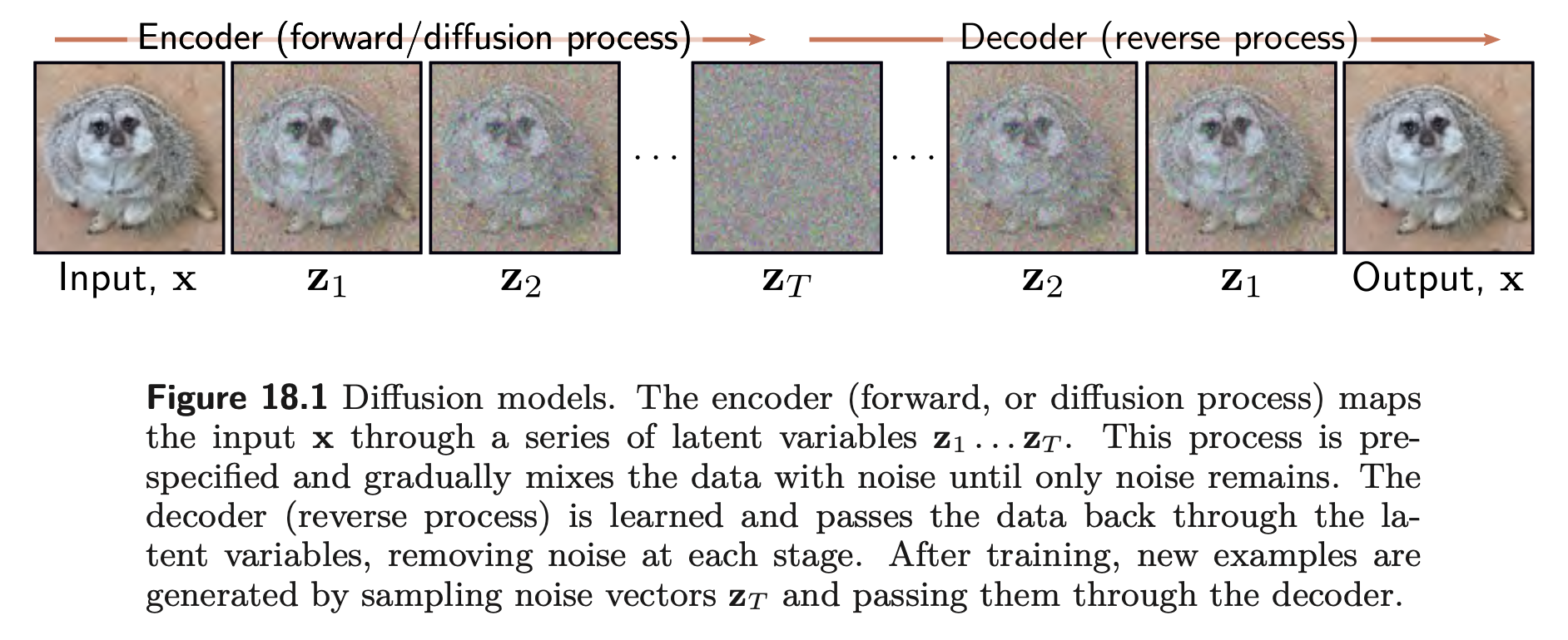
Modern VAEs can produce high-quality samples (figure 17.12d), but only by using hierarchical priors and specialized network architecture and regularization techniques. Diffusion models (chapter 18) can be viewed as VAEs with hierarchical priors... However, in diffusion models, this encoder is predetermined; the goal is to learn a decoder that is the inverse of this process and can be used to produce samples. Diffusion models are easy to train and can produce very high-quality samples that exceed the realism of those produced by GANs.
-
Encoder (forward process)
The encoder is a fixed process that gradually adds noise to the data. With enough time steps, the data becomes a Gaussian noise:determine how quickly the noise is blended and are collectively known as the noise schedule.
- Diffusion kernel
Substituting each step together, all the noise added in each step will be i.i.d. and can be merged as a single noise : where . We can equivalently write this in probabilistic form: - Conditional diffusion distribution This can be computed in closed form since we known the diffusion kernel:
- Diffusion kernel
-
Decoder (reverse process)
where is a neural network that computes the mean of the normal distribution in the estimated mapping from to the preceding latent variable . The terms are predetermined. If the hyperparameters in the diffusion process are close to zero (and the number of time steps is large), then this normal approximation will be reasonable.
- Evidence lower bound (ELBO)
Similar to VAE, the ELBO and its reconstruction interpretation are: - Diffusion loss
The first term measures the probability of reconstructing the original sample ; the second term measures how accurately each denoising step moves the distribution towards the true denoised distributionTo fit the model, we maximize the ELBO with respect to the parameters . We recast this as a minimization by multiplying with minus one and approximating the expectations with samples to give the loss function:
where the first term is the reconstruction term, is the target, mean of , and is the predicted .
- Target reparameterization Therefore, the target (mean of ) can be expressed as:
- Network reparameterization
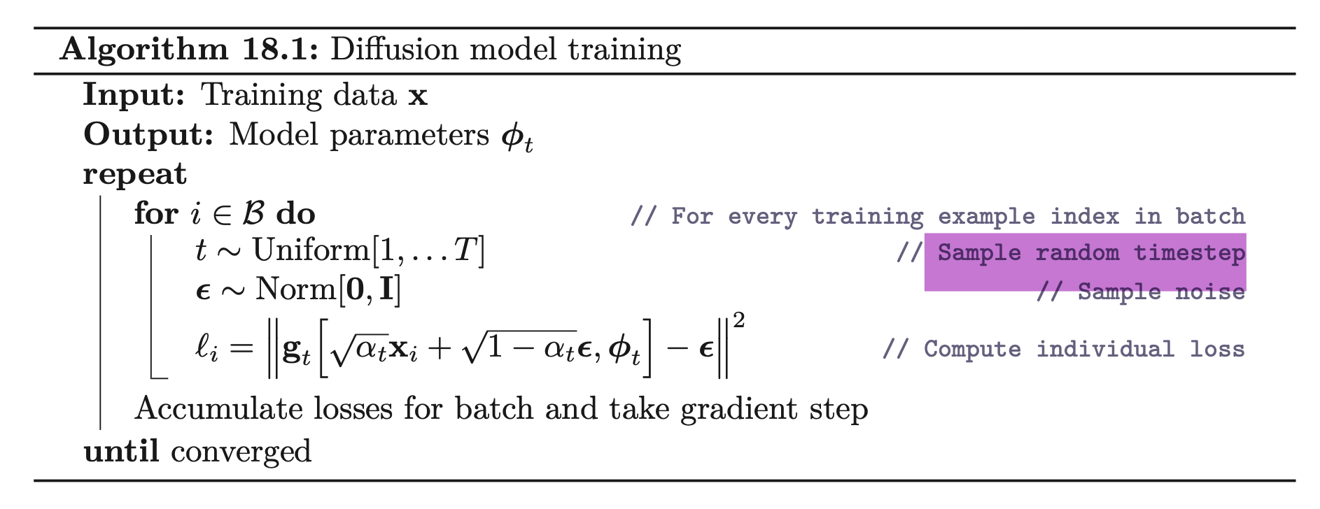
The loss function is modified so that the model aims to predict the noise that was mixed with the original data example to create the current variable... Now we replace the model with a new model , which predicts the noise that was mixed with to create :
- Final form
Substituting the target and network reparameterizations into the loss function and combining the terms, we get: In practice, the scaling factors are ignored:
- Evidence lower bound (ELBO)
-
Implementation
- Training
- Sampling
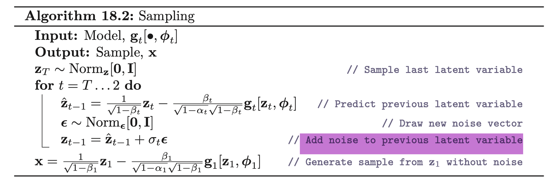
- Applying to images
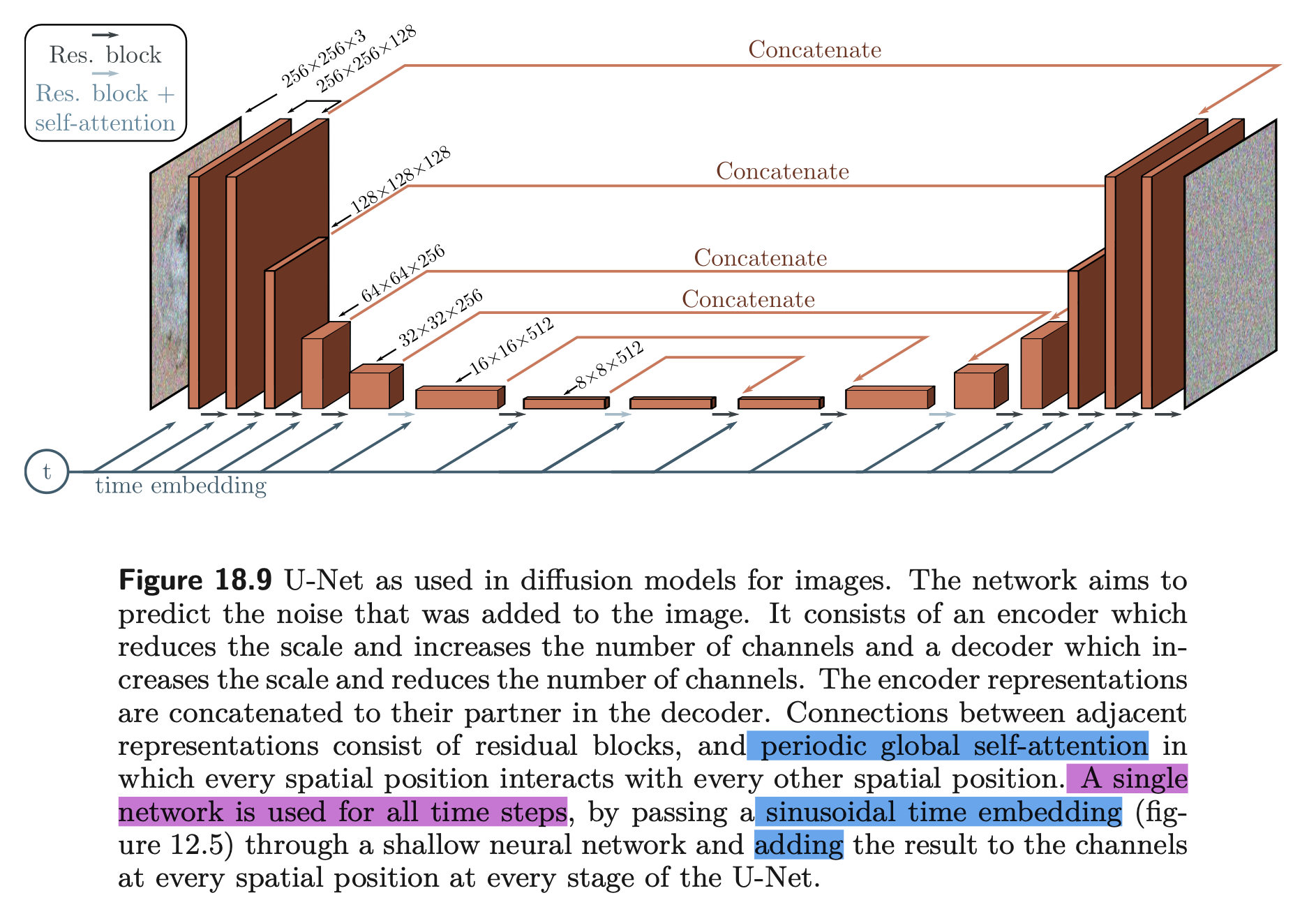
We need to construct models that can take a noisy image and predict the noise that was added at each step. The obvious architectural choice for this image-to-image mapping is the U-Net (figure 11.10). However, there may be a very large number of diffusion steps, and training and storing multiple U-Nets is inefficient. The solution is to train a single U-Net that also takes a predetermined vector representing the time step as input.
- Improving generation speed
The same loss function will be valid for any forward process with this relation, and there is a family of such compatible processes... Among this family are denoising diffusion implicit models, which are no longer stochastic after the first step from x to z1, and accelerated sampling models, where the forward process is defined only on a sub-sequence of time steps. This allows a reverse process that skips time steps and hence makes sampling much more efficient; good sam- ples can be created with 50 time steps when the forward process is no longer stochastic.
- Conditional generation
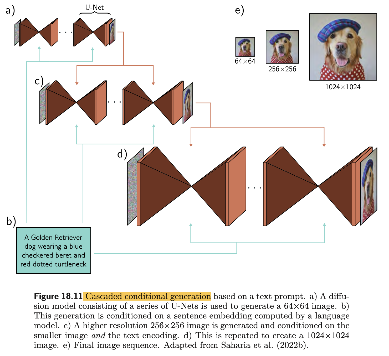
- Classifier guidance
Train a classifier model and use it to calculate the gradient of the log-likelihood of a class label with respect to intermediate code . Add it as an additional term for generating : - Classifier-free guidance
Avoids learning a separate classifier but instead incorporates class information into the main model . In practice, this usually takes the form of adding an embedding based on to the layers of the U-Net in a similar way to how the time step is added.
- Classifier guidance
- Training
Part IV. Reinforcement learning
-
Markov decision process (MDP)
- State
The state of time - Action
The action of time- Policy
The rules that determine the agent’s action for each state are known as the policy... The environment and the agent form a loop (figure 19.6). The agent receives the state st and reward rt from the last time step. Based on this, it can modify the policy if desired and choose the next action at. The environment then advances to the next state according to and issues a reward according to .
- Optimal policy
If we know the state-action value (see below), we can draw the optimal policy as: where is the optimal state-action value.Some reinforcement learning algorithms are based on alternately estimating the action values and the policy
- Policy
- Reward
The reward of time (received at time )- Return
The return is the sum of the cumulative discounted future rewards: - State value
State value characterize how “good” a state is under a given policy by considering the expected return: - Action value
Similarly, action value characterize how "good" an action and state are under a given policy by considering the expected return: - Bellman equations Therefore, the relation between the state/action value at time and is:
- Return
- State
-
Tabular reinforcement learning
Here we briefly overview the taxonomy of tabular reinforcement learning algorithms. In tabular reinforcement learning, the state and action spaces are discrete and small enough to allow for explicit representation of the value functions and policies in tables. More details are documented in the following sections- Model-based methods
Model-based methods use the MDP structure explicitly and find the best policy from the transition matrix Pr(st+1|st,at) and reward structure r[s,a]. If these are known, this is a straightforward optimization problem that can be tackled using dynamic programming. If they are unknown, they can (in principle) be estimated from observed MDP trajectories.
- Model-free methods
Model-free methods assume that the transition matrix and reward structure of the underlying MDP are unknown.
- Value-estimation methods
Value estimation approaches estimate the optimal state-action value function and then assign the policy according to the action in each state with the greatest value.
- Policy estimation methods
Policy estimation approaches directly estimate the optimal policy using a gradient descent technique without the intermediate steps of estimating the model or values.
- Value-estimation methods
- Model-based methods
Model-based dynamic programming
Dynamic programming algorithms assume we have perfect knowledge of the transition and reward structure... The state values are initialized arbitrarily (usually to zero). The deterministic policy is also initialized (e.g., by choosing a random action for each state). The algorithm then alternates between iteratively computing the state values for the current policy (policy evaluation) and improving that policy (policy improvement).
Policy evaluation: We sweep through the states , updating their values:
where is the successor state and is the state transition probability. Each update makes consistent with the value at the successor state using the Bellman equation for state values (equation 19.9). This is termed bootstrapping.
Policy improvement: To update the policy, we greedily choose the action that maximizes the value for each state:
This is guaranteed to improve the policy according to the policy improvement theorem.
Model-free value-estimation
-
Monte Carlo methods
Monte Carlo methods simulate many trajectories through the MDP for a given policy to gather information about how to improve this policy... The action value for a given state-action pair under the current policy is estimated as the average of the empirical returns (i.e., cumulative sums of time-discounted rewards) that follow each time this pair occurs (figure 19.11b).
- On policy method
Then the policy is updated by choosing the action with the maximum value at every state.
- Off-policy method
In off-policy methods, the optimal policy π (the target policy) is learned based on episodes generated by a different behavior policy . Typically, the target policy is deterministic, and the behavior policy is stochastic (e.g., an epsilon-greedy policy).
- On policy method
-
Temporal-difference (TD) methods
Temporal difference (TD) methods update the policy while the agent traverses the MDP.
In both SARSA and Q-learning, the state-action value is updated based on the difference between the current estimate and the estimate after taking a single step
- SARSA (State-Action-Reward-State-Action)
SARSA (State-Action-Reward-State-Action) is an on-policy algorithm with update:
where is the learning rate. The bracketed term is called the TD error and measures the consistency between the estimated action value and the estimate after taking a single step.
- Q-Learning
By contrast, Q-Learning is an off-policy algorithm with update (figure 19.12):
where now the choice of action at each step is derived from a different behavior policy .
-
Deep Q-Networks (DQNs)
In fitted Q-learning, the discrete representation of the action values is replaced by a machine learning model , where now the state is represented by a vector rather than just an index. We then define a least squares loss based on the consistency of adjacent action values (similar to the loss in Q-learning, see equation 19.15):
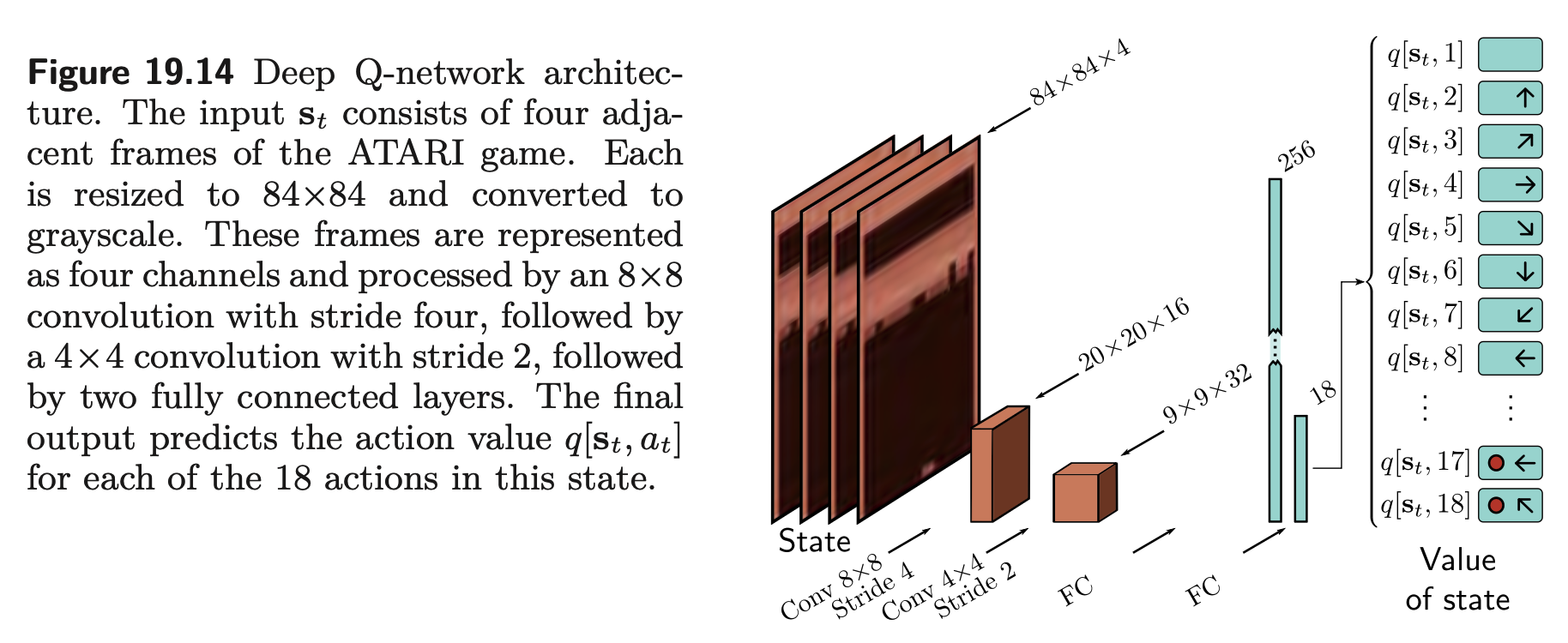
-
Double DQNs
The problem of DQNs is that the same network both selects the target (by the maximization operation) and updates the value: it only updates the action value of the action that is currently estimated to be the best, leading to a systematic bias that overestimates the action values. Double DQNs use two networks to decouple the selection and evaluation of the target action value: selects the action to update , and vice versa
-
- SARSA (State-Action-Reward-State-Action)
Model-free policy-estimation
-
Monte-Carlo policy estimation
-
Gradient-based policy estimation
Consider a trajectory through an MDP. The probability of this trajectory depends on both the state evolution function and the current stochastic policy :
Policy gradient algorithms aim to maximize the expected return over many such trajectories:
where the return is the sum of all the rewards received along the trajectory. To maximize this quantity, we use the gradient ascent update:
where is the learning rate.
- Monte-Carlo approximation
We want to approximate this integral with a sum over empirically observed trajectories. These are drawn from the distribution , so to make progress, we multiply and divide the integrand by this distribution:
This equation has a simple interpretation (figure 19.15); the update changes the parameters to increase the likelihood of an observed trajectory in proportion to the reward from that trajectory. However, it also normalizes by the probability of observing that trajectory in the first place to compensate for the fact that some trajectories are observed more often than others. If a trajectory is already common and yields high rewards, then we don’t need to change much. The biggest updates will come from trajectories that are uncommon but create large rewards.
- Final form
The equation can be further simplified by the likelihood ratio identity : Combining with the (non-obvious but proven) fact that the rewards before time does not affect the update after time :
- Monte-Carlo approximation
-
State-dependent baseline subtraction
Some actions have greater value simply because the state yields higher rewards, rather than being truly better than other actions. To avoid this bias, we can subtract a baseline from the return:Here, we are compensating for variance introduced by some states having greater overall returns than others, whichever actions we take. A sensible choice is the expected future reward based on the current state, which is just the state value . In this case, the difference between the empirically observed rewards and the baseline is known as the advantage estimate. Since we are in a Monte Carlo context, this can be parameterized by a neural network with parameters , which we can fit to the observed returns using least squares loss:
-
-
Temporal difference policy estimation (actor-critic methods)
Actor-critic algorithms are temporal difference (TD) policy gradient algorithms... Often the same network represents both actor and the critic, with two sets of outputs that predict the policy and the values, respectively... The agent typically collects a batch of experience over many time steps before the policy is updated.
- Critic
Similar to state-dependent baseline method, the critic is a neural network that estimates the state value , i.e. the critic. It's characterized by network parameters and is trained (or bootstrapped) with: - Actor
The policy network that predicts is termed the actor:In the TD approach, we do not have access to the future rewards along this trajectory. Actor-critic algorithms approximate the sum over all the future rewards with the observed current reward plus the discounted value of the next state:
Here the value is estimated by a second neural network with parameters . Substituting this into equation 19.38 gives the update:
- Critic