Spectral Mesh Processing | Bruno Lévy & Hao Zhang

Spectral mesh processing | ACM SIGGRAPH 2010 Courses

A gentle introduction

• Setting the stage
  Laplacian, Laplacian smoothing and its relationship with midpoint smoothing
• Spectral transform
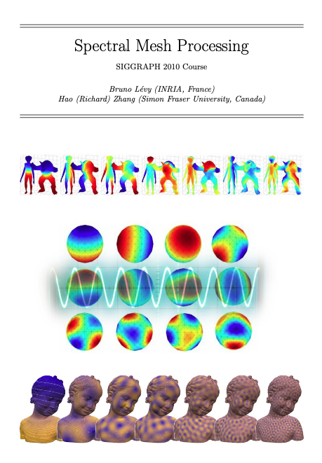
  Use eigenvectors of the laplacian as the basis to represent coordinates functions $x(i), y(i)$.

  From linear algebra, we know that since L is symmetric, it has real eigenvalues and a set of real and orthogonal set of eigenvectors which form a basis. Any vector of size n can be expressed as a linear sum of these basis vectors.

  • Signal reconstruction and compression with this basis
    As well as filtering and smoothing
  • Connection with discrete Fourier transform

    The connection we seek, between DFT and spectral analysis with respect to the Laplace operator, is that the DFT basis functions, the $g_k$’s, form a set of eigenvectors of the 1D discrete Laplace operator $L$, as defined in (3). A proof of this fact can be found in Jain’s classic text on image processing [Jai89], where a stronger claim with respect to circulant matrices was made.

• P.S. The eigenvectors of a symmetric matrix are orthonormal, thus ideal for being used as functional basis.
  linear algebra - Eigenvectors of real symmetric matrices are orthogonal - Mathematics Stack Exchange

Fourier analysis for meshes

• Fourier analysis on 1D function:
  $f(x) = \sum_{k=0}^{\infty} \tilde f_k H^k(x)$ where $\tilde f_k$ is given by the inner product $\langle f, H^k \rangle = \int_0^1 f(x) H^k(x) dx$.
• Noted that the functions $H^k$ of the Fourier basis is the eigenfunctions of $-\partial^2/\partial x^2$.

  This construction can be extended to arbitrary manifolds by considering the generalization of the second derivative to arbitrary manifolds, i.e. the Laplace operator and its variants.

  • The discrete setting: Graph Laplacians
  • The Continuous Setting: Laplace Beltrami
    $\Delta = \text{div grad} = \nabla \cdot \nabla = \sum_i \frac{\partial^2}{\partial x^2_i}$
    • With exterior calculus (EC)
      $\Delta = \text{div grad} = \delta d = \sum_i \frac{1}{\sqrt{|g|}}\frac{\partial}{\partial x_i} \sqrt{|g|}\frac{\partial}{\partial x_i}$

      The additional term $|g|$ can be interpreted as a local ”scale” factor since the local area element $dA$ on $\mathcal S$ is given by $dA = \sqrt{|g|} dx_1 \wedge dx_2$.

Discretizing the Laplace operator

This chapter provides two ways to discretize the Laplace operator, both are quite dense and require certain math prerequisites.

• The FEM Laplacian
• The DEC Laplacian

Computing eigenfunctions

• Issues with typical iterative eigenfunctions solvers
  • Iterative solvers performs much better for the the eigenvectors associated with large eigenvalues, whereas for spectral mesh processing we are more interested in the eigenvectors associated with small eigenvalues.
  • Computation time is super-linear in the number of requested eigenpairs, which makes mesh with thousands of vertices infeasible.
• Shift-invert spectral transform
  The original eigenvalue decomposition problem:
  $\overline \Delta \overline H^k = \lambda_k \overline H^k$
  After shift-invert spectral transform:
  $\Delta^{SI} = (\overline D - \lambda_S Id)^-1 \Rightarrow \Delta^{SI} \overline H^k = \mu_k \overline H^k$
  where $\lambda_k = \lambda_S + 1/\mu_k$.

Applications

• Use of eigenvectors
  • Parameterization and remeshing
  • Clustering and segmentation
  • Shape correspondence and retrieval
• Use of spectral transforms

  Conceivably, any application of the classical Fourier transform in signal or image processing has the potential to be realized in the mesh setting.

  • Geometry compression
  • Watermarking