Computer Vision: Algorithms and Applications | Richard Szelisky

Free official electronic version: Computer Vision: Algorithms and Applications, 2nd ed.

P.S. Part name was added by me.

Introduction

• Sample Editor Command
  Very difficult due to imperfect information.
• A brief history of computer vision.

Part I: The Basics

Image formation

• Sample Editor Command
  Homogeneous coordinates and how to use it to describe 2D/3D transformation compactly.
• Photometric image formation
  Models of lighting, reflectance, shading, and optics.
• Digital camera
  • Sampling and aliasing when digitizing image.
  • Demosaicing color filter arrays and describe colors in different color space.
  • Gamma correction and white balance.
  • Image compression technique used by JPEG and other image formats.

Image processing

• Operations
  • Point-level operators
  • Convolutional operators (linear filtering)
  • Neighborhood operators
    e.g. Bilateral filtering
• Pyramids
  • Fourier transforms
  • Laplacian pyramids
  • Wavelets pyramids

Model fitting and optimization

• Data interpolation
  • Radial basis functions (RBFs)
    When using robust loss function, the data fitting process is called robust data fitting.
  • Variational methods
    Optimize a function directly by regularizing its derivatives via energy minimization.
• Markov random fields
  Honestly, since the book doesn't cover the preliminary knowledge, I don't quite understand this part.

Deep Learning

• Classical machine learning
  • Supervised learning
    e.g. Nearest neighbors, Bayesian classification, logistic regression, support vector machine, and decision trees (forests).
  • Unsupervised learning
    e.g. Clustering, K-means (vs Gaussians mixture), principal component analysis, and manifold learning (non-linear dimensionality reduction).
  • Semi-supervised learning
• Deep neural networks
  • Basics components of MLP
    Layers, weights initialization (e.g. He Initialization), activations (e.g. ReLU), regularization (e.g. dropout), normalization (e.g. Batch Normalization), loss function, and back-propagation.
  • CNN and its variants
    e.g. AlexNet, GoogLeNet, ResNet, VGGNet-16, ZF Net, etc.
    • Adversarial examples
    • Self-supervised learning
      e.g. Pre-training and contrastive learning.
    • 3D CNN
  • Other networks: RNN, Transformer, VAE, GAN, etc.

Part II: 2D Vision

Recognition

• Instance recognition
  Recognize objects in a cluttered scene.
• Image classification
  • Classic feature based methods include bag of words and part-based models, etc.
  • Classic (PCA) decomposition based methods include Active Appearance Model and 3D Morphable Model, etc.
  • Starting from AlexNet, Deep Learning based methods have taken the field.
• Object detection
  When subpart of the image is localized and classified, it's called object detection.
  • Classic methods are typically based on PCA, clustering, support vector machine, boosting, etc.
  • Seminal works based on Deep Learning include YOLO, R-CNN, Fast R-CNN, Faster R-CNN, FPN, DETR, etc.
• Semantic segmentation
  When classification is down to pixel-level, it's called semantic segmentation.
  Seminal works include U-Net, Mask R-CNN, etc. More recent works tends to adopt feature pyramid based framework.
  • When instance boundary is distinguished, it's called instance segmentation.
  • Seminal works of human pose estimation include OpenPose, DensePose, and HRNet, etc.
• Video understanding
  e.g. Two Stream CNN
• Vision and language
  e.g. CLIP, DALL·E, VQA, etc.

Feature detection and matching

• Point and patch-level
  • Feature detector
    Using auto-correlation to find the most distinguishable feature points from the image.
    • Uncertainty indicator, asymmetry indicator, and Gaussian weighting window, scale pyramids are common techniques to augment it.
    • Scale (e.g. SIFT), rotation (e.g. Haris), and affine (e.g. MSER) invariance are also addressed.
  • Feature descriptor
    e.g. Scale Invariant Feature Transform (SIFT)
  • Feature matching
    To improve efficiency, hashing, K-d tree, bin, etc. are applied.
    To improve robustness, RANSAC can be used.
• Edge and contour-level
  • Edge detection
    Laplacian of Gaussian (LoG) or Difference of Gaussian (DoG) and then find the zero crossing.
  • Contour detection
    Linking neighboring detected edges pixels.
    When the contour is detected interactively via energy minimization scheme, it's called contour tracking. e.g. Snake, scissors, level sets, etc.
  • Lines and vanishing points
    e.g. Hough transforms
• Segmentation
  The image features can also be used to merge/segment image regions.
  e.g. Region merging, watershed, mean shift, normalized cuts, etc.

Image alignment and stitching

• Pairwise alignment
  With a pre-defined motion model, the parameters that best align two image can be estimated via least squares. For better results, iterative algorithms like non-linear least squares can be use. Further improvements can be achieved via robust least squares and RANSAC.
  • Jacobian $J$: $\Delta x = x' - x = \frac{\partial f}{\partial p}p = J(x)p$
  • Hassian $H$: $H(x) = \sum_i J^T(x) J(x)$
• Global alignment (bundle adjustment)
  When directly optimizing the alignments of all images instead of a pair of images, it's called bundle adjustment. It can be formulated as summed cost of all pairs of images (features correspondence) and optimized via least squares.
• Compositing
  When compositing aligned images, multiple available pixels of a compositing location need to be select or weighted for deghosting. Exposure compensation is also needed.

Motion estimation

• Parametric motion
  Brightness and color difference are also taken into account.
  • Translational motion model
    Classic motion estimation techniques include hierarchical motion estimation, Fourier-based alignment, incremental refinement based on Taylor series expansion for sub-pixel level.
    • Optical flow constraint (Lucas-Kanade)
      $I_x u + I_y v + I_t = 0$
  • Motion model w/ more params Taylor series expansion and gradient descent/non-linear least squares.
    Can be optimized with
  • Spline-based motion
    Define motion based on some control vertex.
• Optical flow
  Motion of each pixel - a highly under-constrained problem.
  • Regularization-based method
    Smoothness term can be used to constrain the motion field. Markov random field (MRF) is another alternative.
  • Patch-based method
    Performs translational alignment within a coarse-to-fine pyramid.
  • Deep Learning-based methods
    e.g. DeepFlow, FlowNetS, SPyNet, PWC-Net, $\text{HD}^3$, LiteFlowNet3, etc.
• Layered motion
  Group pixels into layers/objects.

Computational photography

• Photometric calibration
  Covers radiometric response function (log exposure > pixel value), noise level estimation, vignetting, and optical blur.
• High dynamic range imaging (HDR)
  Merging photos taken under different exposures. When displaying a HDR image, it needs to be tune mapped to a displayable gamut, for which sophisticated methods utilizing high/low-pass filters, gradient information, etc. are developed.
• Image quality improvement
  Covers super-resolution, denoising, and blur removal.
  Image demosaicing and lens blur (bokeh) are also discussed.
• Image matting and compositing
  Covers blue screen matting, natural image matting, optimization-based matting, and video matting.
  Matting with special effects like smoke, shadow, and flash are also discussed.
• Texture analysis and synthesis
  Can be used f/ hole filling, non-photorealistic rendering, style transfer, etc.

Part III: 3D Vision

Structure from motion and SLAM

• Geometric calibration
  Point $p$ in 3D space is mapped to the camera's local frame by extrinsic: $[R|t]p$, and then mapped to the pixel grid by intrinsic: $K[R|t]p$.
  • Camera intrinsic estimation
    The most important factor of camera intrinsic is its focus length. For wide angle lens, the radial distortion factors are also needed.
  • Camera extrinsic estimation (pose estimation)
    With known point locations, the camera extrinsic can be estimated via least squares or iterative optimization.
  • $\infty$ Triangulation
    The converse problem of pose estimation is estimate a point's location with known camera pose.
• Structure from motion (SfM)
  SfM aims at recovering the corresponding points locations in space as well as the cameras poses at the same time.
  • Epipolar geometry
    
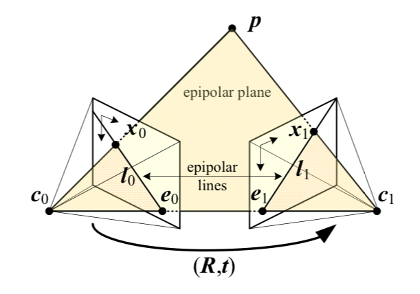
    • Points in $l_0$ is mapped to $l_1$ when viewed from camera 1.
    • Essential matrix $E = [t]_{\times} R$
      Epipolar constraint: $\hat{x}_1^T E \hat{x}_0 = 0$
    • Fundamental matrix $F = K_1^{-T}EK_0^{-1}$
      When camera intrinsic is unavailable, then the 3D locations of the pixels are unavailable. In this case, the equation can only be formulated with the pixel grid coordinates: $x_1^T F x_0 = 0$
  • Two-frame SfM
    Based on epipolar constraint, 8-point algorithm uses 8 pairs of corresponding points to estimate the extrinsic as well as the 3D point locations.
  • Multi-frame SfM
    Bundle adjustment can be used in the context of 3D and for SfM, leading to multi-frame SfM. For efficiency, sparsity structure can be exploited.
• Simultaneous localization and mapping (SLAM)
  Solving the (sparse) 3D reconstruction and localization problem online. It's extensively applied in autonomous navigation and augmented reality (AR).

Depth estimation

• Plane sweep
  Based on epipolar geometry, warp source image $k$ to disparity plane $d$ of a virtual camera to form a disparity space image (DSI) $\tilde{I}(x, y, d, k)$, and then use the DSI for dense depth estimation.
  • Rectification
    Based on epipolar geometry, rectify images to for dense matching.
  • Local optimization
    Using window-based aggregation of the matching cost on DSI to optimize the depth estimation.
  • Global optimization
    Using global optimization methods like dynamic programming to optimize the depth estimation on DSI.
• Multi-view stereo
  Depth estimation with multiple views.
  e.g. COLMAP (used by NeRF).
• Monocular depth estimation
  Depth estimation with single view. Usually based on Deep Learning.

3D reconstruction

• Surface representations
  e.g. Triangle mesh, point cloud, voxels, implicit functions/signed distance function, etc.
• Shape from X
  Recover shape from shading, texture, focus, etc.
  • 3D scanning
    Active (illumination) stereo: light detection and ranging (Lidar), laser-based 3D scanners, time-of-flight (ToF), etc.
  • Model based reconstruction
    With shape model as prior, the reconstruction can be much more accurate and efficient. It has been widely used on architecture, face (e.g. FLAME), hand (e.g. MANO), human body (e.g. SMPL, SMPL-X, STAR), etc.
• Recovering texture maps and albedos
  • Texture maps
    Texture maps can be constructed after parametrizing the surface with $(u, v)$ coordinates.
  • Albedo maps
    Light source can be explicitly modeled to estimate the reflectance component (albedo) maps as well as making the texture map estimation more accurate.
  • Bidirectional reflectance distribution functions (BRDFs)
    
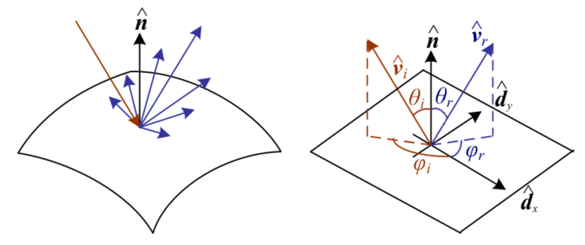
    For view-dependent appearance modeling.

Image-based rendering

• Image-based rendering (view interpolation)
  • View-dependent texture maps
    Attach multiple texture maps on the shape for different view angles and blend these texture in rendering.
  • Layered depth images
    Represent scene as layers of different depth. This idea is rediscovered recently as multiplane image (MPI).
  • Lumigraphs
    The light color of a ray crossing two points from two planes bounding the 3D volume.
  • Light fields
    The emitted light color of any point in a 3D volume.
  • $\infty$ Environment mattes
    Instead of changing the virtual camera, environment mattes changes background.
• Video-based rendering
  • Video animation
    Animate an image with newly specified activity/script.
  • Video textures
    Continue the video in a plausible manner.
  • 3D and free-viewpoint video
• Neural rendering w/ Deep Learning
  Survey: TewariA2020
  These methods can be classified by their 3D representations: textured-mapped mesh, depth images and layers, volumetric grids (e.g. NeRF, NeRF in the wild, etc.), and implicit functions (e.g. NeuS).

Conclusion

• Computer vision is a board field without unifying principles, due to its expansive definition as well as the incredible complexity inherent in the formation of visual information.
• Physical principles, statistical methods, and machine learning are the major foundations of computer vision.
  • Why learn pre-deep learning techniques? Shree Nayar explained:
    • When you can solve a problem elegantly via first principles, it doesn't worth it to collect massive amount of data to do deep learning.
    • When a network doesn't work, first principles are what you have only, and probably your only hopes to understand why.
    • Finally, curiosity is a human nature.
• Future directions of the field.

Appendix

Linear algebra and numerical techniques

• Matrix decompositions
  • Singular value decomposition (SVD)
    $A_{m \times n} = U_{m \times p} \Sigma_{p \times p} V_{p \times n}^T$
    $AV = U\Sigma \Leftrightarrow A v_j = \sigma_j u_j$
    $A = \sum_j \sigma_j u_j v_j^T$
    • Eigenvalue decomposition
      Symmetric matrix $C = U \Lambda U^T$
      • Principle component decomposition (PCA)
        $C = \frac{1}{n} \sum_i (x_i - \overline{x}) (x_i - \overline{x})^T$
  • QR factorization
    $A = QR$
  • Cholesky factorization
    $C = L L^T = R^T R$
• Least squares
  • Linear least squares
    • Vertical residuals
      $E = \|Ax - b\|^2 = x^T(A^TA)x - 2 x^T (A^T b) + \|b\|^2$
      $\arg\min_x E \Rightarrow \frac{\partial E}{\partial x} = 0 \Rightarrow A^T A = A^T b$
      Perform Cholessky factorization on $A^T A = R^T R$, then the optimized $x$ can be solved by solving $\begin{cases}R^Tz = d\\Rx=z \end{cases}$
    • Total residuals
      $E = \|Ax\|^2 = x^T (A^T A) x$
      $\arg\min_x x^T (A^T A) x$ s.t. $\|x\| = 1$
      The optimized $x$ should be the eigenvector associates with the smallest eigenvalue of $A^T A$.
  • Non-linear least squares
    Estimate the iterative increment $\Delta p$ via Taylor series expansion:
    $E(\Delta p) = \sum_i \|J(x_i,p)\Delta p - r_i\|$
    $p \leftarrow p + \alpha \arg\min_{\Delta p} E$
    Important variants include Damped Gauss-Newton algorithm, Levenberg-Marquardt algorithm, etc.
• Efficiency tricks
  • Direct sparse matrix techniques
    e.g. Variable reordering.
  • Iterative techniques
    e.g. Conjugate gradient, preconditioning, multi-grid, etc.

Bayesian modeling and inference

• Estimation theory
  Introduce the likelihood of measurement noise under the setting of multivariate Gaussian noise.
  • Mahalanobis distance $\|y_i - \overline{y}_i\|_{\Sigma_i^{-1}}$
  • Negative log likelihood $-\log L$
  • (Fisher) information matrix (the inverse covariance) $C_i = \Sigma^{-1}$
• Inference
  • Maximum likelihood
    Via (robust) least squares.
  • Bayesian inference
    $p(x|y) = \frac{p(y|x)p(x)}{p(y)} \Rightarrow -\log p(x|y) = -\log p(y|x) - \log p(x) + \log p(y)$
  • Markov random field
    Use Gibbs or Boltzmann distribution to describe the prior probability $p(x)$, with negative log likelihood being written as sum of pairwise interaction potentials.
• Uncertainty (error) estimation

Supplementary material

Important datasets, benchmarks, softwares, and lectures.